A Databricks streaming table can process data incrementally without running continuously. Confusing those two decisions is an expensive mistake.
Continuous Lakeflow pipelines can incur unnecessary compute costs when their configured freshness exceeds actual business requirements. A pipeline with a 15-minute freshness requirement, for example, does not necessarily need compute available continuously. If the source is quiet for long periods, executors spend most of their time waiting while the pipeline continues paying for that availability. This often happens when teams choose continuous execution during launch to meet freshness requirements but never revisit the execution model as usage patterns become clearer.
Databricks cost reviews tend to focus on oversized clusters. That matters, but it is often not the largest mistake in a Lakeflow pipeline. The more consequential problem can sit one level above node size: the execution lifecycle does not match the latency the business actually uses.
The phrase “always-on streaming table” also hides a technical distinction. A Databricks streaming table defines how data is processed. Continuous and triggered modes define how the pipeline runs. Databricks supports streaming tables and materialized views in either pipeline mode, and standalone streaming tables and materialized views are always refreshed in triggered mode. Lakeflow pipelines were called Databricks DLT (Delta Live Tables) until June 2025, when Databricks renamed the product Spark Declarative Pipelines on Lakeflow.
A Databricks streaming table therefore does not need to run continuously to remain incremental. The better question for Databricks cost optimization is: What is the least expensive execution pattern that still satisfies the measured freshness requirement?
Do Databricks streaming tables need to run continuously?
No. A Databricks streaming table records its progress through checkpoints, so it processes data incrementally in either of its two modes: triggered or continuous.
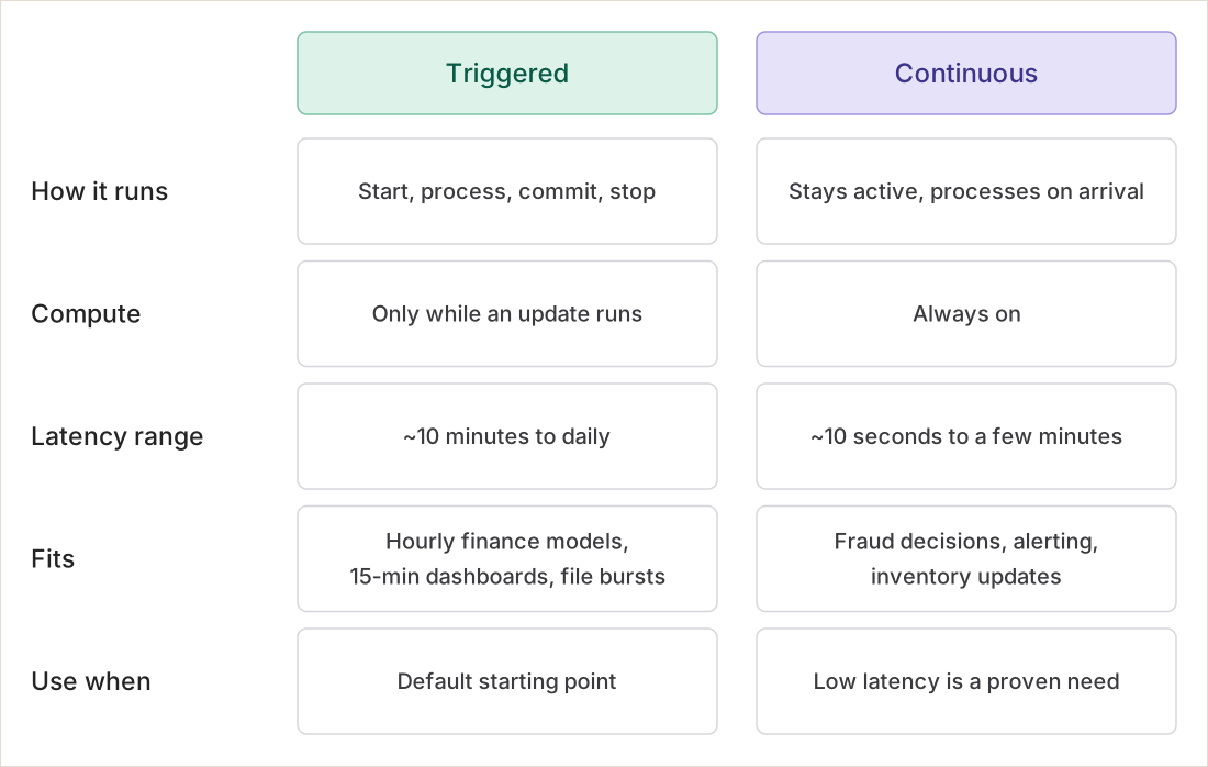
In triggered mode, the pipeline starts, processes the data available when the update begins, commits its progress, and stops. The next update resumes from that checkpoint. It does not need to replay the complete source history.
Continuous mode keeps the pipeline active and processes new data as it arrives. This reduces the delay between arrival and processing, but it also requires continuously available compute.
Those modes solve different problems.
Triggered execution fits an hourly finance model, a fifteen-minute operations dashboard, or a source that lands files in periodic bursts.
Continuous execution fits fraud decisions, alerting, inventory updates, and other workloads where seconds of delay change an operational outcome.
Databricks recommends starting with triggered execution because it consumes compute only while an update is running. Continuous execution should be reserved for workloads with a demonstrated low-latency requirement. The current guidance from Databricks places triggered pipelines roughly in the ten-minute-to-daily range and continuous pipelines in the ten-second-to-few-minute range. Real-time mode covers operational workloads that require sub-second processing.
These time ranges are useful starting points, but they are not substitutes for measuring the actual data path.
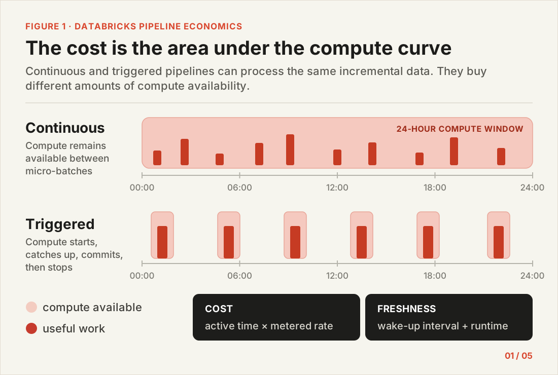
Figure 1. Continuous execution buys a shorter wait between data arrival and processing. The cost is the full span of time for which compute remains available, not only the periods where useful work occurs.
When do Databricks streaming tables need continuous mode?
Continuous compute keeps a pipeline running at all times so it can process data as soon as it arrives. You pay for that compute whether or not the consumer needs data that quickly. Sometimes the consumer does. If an authorization system needs a risk signal within 30 seconds, a pipeline scheduled every 10 minutes will not meet the requirement.
Costs become a problem in two cases. First, the pipeline stays in continuous mode after the consumer no longer needs low latency. Second, a single low-latency table forces every upstream table it depends on, across the Bronze, Silver and Gold layers, to run in continuous execution too.
A production design needs an explicit freshness service-level objective (SLO), measured from source event time to data being available to the consumer. Measure this at P50 and P95. Include each step that adds delay: source delay, queueing, compute startup, checkpoint recovery, processing, commit time, downstream publication, and dashboard caching.
"Real time" is not a specific enough requirement to work with. A 5-second target, a 5-minute target and a 1-hour target each need a different pipeline design. Choose the pipeline mode based on the consumer's freshness requirement and the data's arrival pattern, not on the dataset type (streaming table or materialized view).
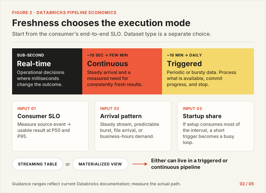
Figure 2. Choose execution mode from the consumer’s freshness SLO and the arrival pattern. Dataset type and execution mode are independent decisions.
Most of the DBU cost of continuous mode comes from uptime
Consider a continuous pipeline that consumes an average of 6 DBUs per wall-clock hour. The number is illustrative. An actual evaluation should use billing records from the target pipeline.
Running continuously for a year produces:
6 DBU/hour × 24 hours/day × 365 days = 52,560 DBUs/yearNow assume the consumers only need data refreshed once an hour. Historical runs show that each triggered update finishes in fifteen minutes. After tightening the compute envelope, the pipeline consumes an average of 3 DBUs per active hour.
The annual consumption becomes:
3 DBU/hour × 0.25 active hours/run × 24 runs/day × 365 days = 6,570 DBUs/yearThe modeled reduction is 45,990 DBUs, or 87.5%. The triggered design uses one-eighth as many DBUs.
| Execution mode (illustrative model) | Refresh | Active compute per day | Average DBUs per active hour | DBUs per year |
|---|---|---|---|---|
| Continuous | Always on | 24 hours | 6 | 52,560 |
| Triggered, hourly | Once an hour, 15-minute update | 6 hours | 3 | 6,570 (87.5% fewer) |
Not every continuous pipeline can save 87.5%. The example changes two variables:
The number of hours for which compute remains active.
Average DBU consumption during those active hours.
Startup overhead, source volume, pipeline complexity, autoscaling behavior, performance mode, retries, and the actual duration of each update will change the result.
The formula is:
annual platform cost = metered DBUs × effective DBU rateFor classic compute, the underlying cloud infrastructure charge must be added separately. A list-price estimate can be produced by joining system.billing.usage to system.billing.list_prices, as in this breakdown of Databricks compute costs. A realized-savings calculation should use the effective rate in the organization’s Databricks contract.
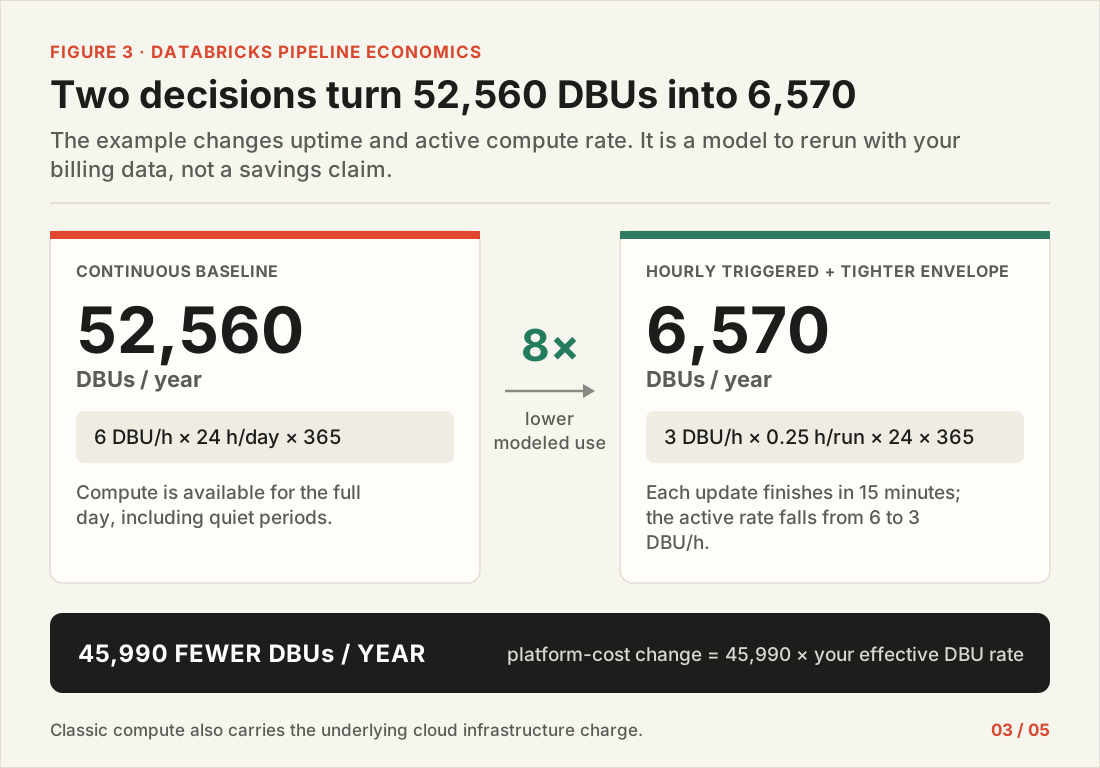
Figure 3. The eight-fold result is an illustrative model, not a benchmark. Recompute it with the pipeline’s observed DBUs, active duration, schedule, and effective price.
Five-minute triggered schedules can be worse than continuous mode
Replacing every continuous pipeline with a triggered one would create a different set of problems. At short intervals, triggered execution repeatedly pays for compute provisioning, runtime initialization, graph setup, source connections, checkpoint recovery, and teardown.
A Databricks employee benchmark compared a serverless pipeline scheduled every five minutes with the same workload running continuously. Each triggered lifecycle took between 153 and 194 seconds, averaging about 177 seconds. Continuous execution reduced median freshness from 4.0 minutes to 33 seconds and P95 freshness from 9.3 minutes to 60 seconds. Eligible streaming queries also saw roughly 1.7 times the throughput through stream pipelining.
That is one vendor-run benchmark on one workload, not a universal performance result. If a five-minute schedule spends nearly three minutes starting, processing, and stopping, the pipeline has become a busy loop with poor freshness. Continuous execution may be the better architecture and, at sufficient utilization, may not be the more expensive one.
There is also more room between the two extremes than the pipeline-mode toggle suggests. For continuous pipelines, pipelines.trigger.interval controls how frequently an individual flow begins an update. Current defaults vary by flow type:
Five seconds for streaming queries.
One minute for complete queries over Delta sources.
Ten minutes when complete queries may use non-Delta sources.
The interval can be configured at the table level when flows have different requirements.
Serverless performance mode also changes the trade-off. Standard mode is intended for cost-sensitive batch work and typically starts in four to six minutes. Performance-optimized mode starts in seconds and is designed for latency-sensitive execution. An hourly pipeline can usually absorb the startup time of Standard mode. A five-minute schedule probably cannot.
The boundary should be found empirically. Plot total active time, startup share, end-to-end freshness, backlog, update duration, and DBUs per unit of data over several representative weeks. The cheapest valid mode is then visible in the data.
Split Lakeflow pipelines where freshness targets differ
Many expensive pipelines are not uniformly latency-sensitive. Bronze ingestion may need new events within thirty seconds. Silver tables may tolerate five minutes. A Gold revenue materialized view may only be read during business hours and can refresh once per hour.
Keeping all three layers in one continuous graph makes the strictest freshness requirement the default for every dataset. That coupling is convenient during development and expensive in production.
Databricks recommends grouping datasets by shared cadence and dependency, then splitting pipelines at ownership, layer, and latency boundaries. Its guidance is direct: a continuous low-latency stream should not share a pipeline with a once-a-day batch aggregate.
A more appropriate design might use:
A continuous ingestion pipeline for the small part of the graph that genuinely requires low latency.
A triggered transformation pipeline for datasets with five- or fifteen-minute requirements.
A separate hourly or daily pipeline for expensive aggregates and reporting tables.
A Lakeflow Job to coordinate dependencies and provide a unified operational view.
This division also allows each pipeline to use the compute model suited to its work. The continuous ingestion path can use serverless execution or enhanced autoscaling tuned for a steady streaming workload. Triggered transformations can use Standard serverless mode or a right-sized classic update cluster that terminates after the update.
Pipelines should not be split mechanically at every medallion-layer boundary. A tightly coupled chain with the same freshness requirement may belong together. The split is justified when independent control over cadence, compute, ownership, or failure blast radius is worth the additional orchestration.
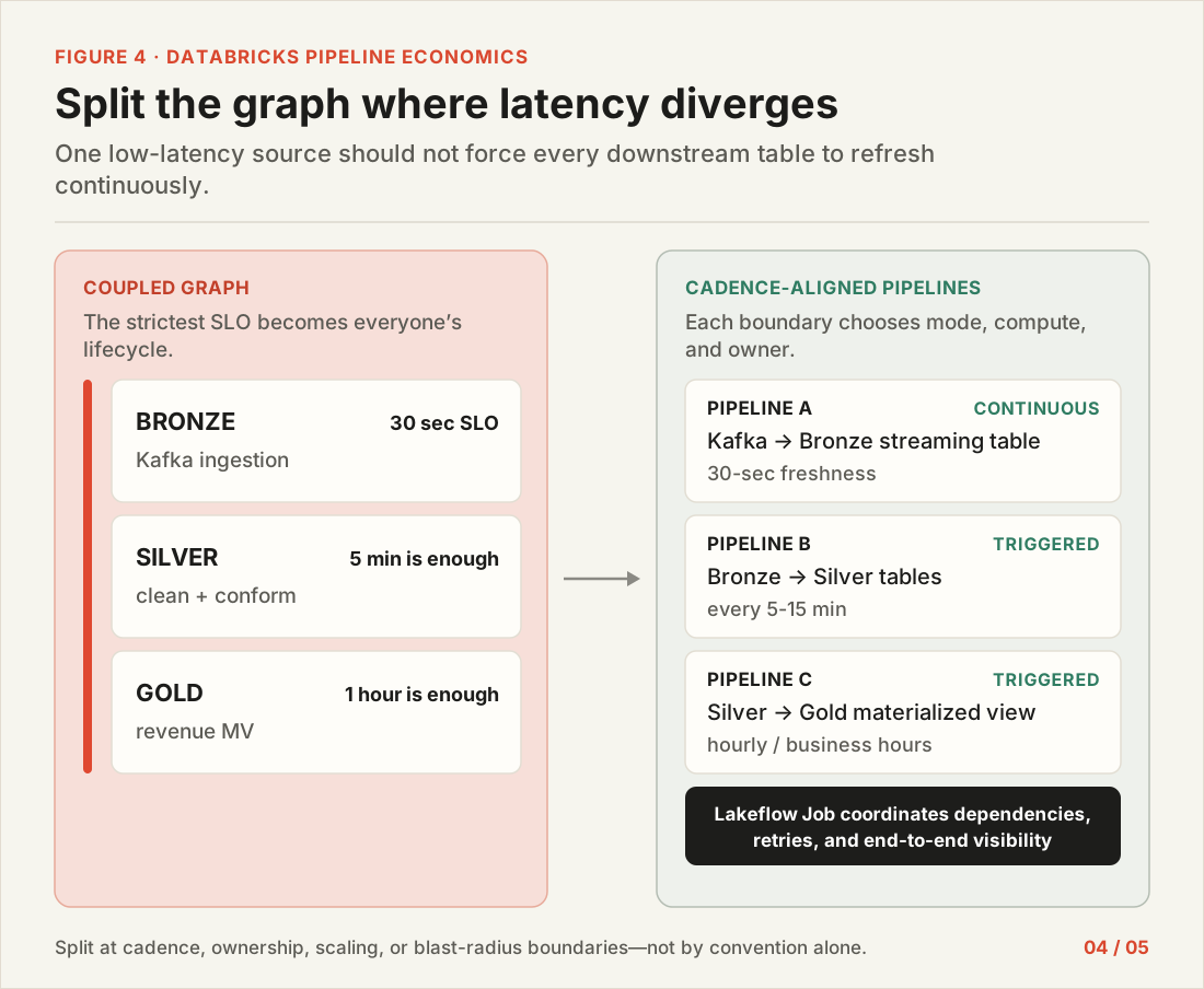
Figure 4. Split the dataflow where freshness, ownership, or scaling requirements diverge. Orchestrate the pipelines together in a Lakeflow Job so the operational view remains coherent.
A cheaper schedule does not fix an expensive refresh plan
Execution mode controls when compute runs. Refresh strategy controls how much data each update processes, and that second decision can cost more than the first.
During a normal refresh, a streaming table processes records that arrived after its previous checkpoint. A full refresh clears the table’s data and checkpoints and reprocesses the source. Its duration and cost can therefore scale with the available source history.
Materialized views have different behavior. They preserve batch-equivalent results and are incrementally refreshed when Databricks can prove that an incremental plan is valid and economical.
On serverless pipelines, Databricks evaluates whether an incremental refresh is possible and uses a cost model to choose between incremental work and full recomputation. Materialized views running on classic pipeline compute are fully recomputed.
Moving a materialized-view pipeline from continuous execution to an hourly schedule may reduce uptime. It does not fix an hourly full scan of a large history.
Use EXPLAIN CREATE MATERIALIZED VIEW before deployment to evaluate structural eligibility for incremental refresh. At runtime, inspect the incrementalization information in the pipeline UI and event log. The event log can report techniques such as ROW_BASED, GROUP_AGGREGATE, NO_OP, and FULL_RECOMPUTE, as well as reasons why the cost model rejected an incremental plan.
The same event log exposes streaming backlog and, for classic pipelines, executor counts, task-slot utilization, and queued tasks. That evidence helps distinguish four problems that may look similar on an invoice:
Continuous compute spending most of its time waiting for data.
A triggered pipeline dominated by startup.
A cluster with an inappropriate autoscaling floor or ceiling.
A materialized view repeatedly scanning more history than expected.
Changing the schedule fixes only the first two.
Storage costs do not scale with refresh frequency
Bronze, Silver, and Gold tables can accumulate substantial storage. Continuous execution is not automatically the cause. Storage consumption is affected by logical data retention, duplicate materializations, unnecessary persisted intermediates, Delta history, Change Data Feed retention, streaming state, checkpoints, and table design.
A pipeline that refreshes every minute and one that refreshes every hour should converge to the same logical table contents if they process the same input correctly. Refresh frequency can affect checkpoint and transaction-log churn, small-file patterns, maintenance activity, and how quickly data becomes eligible for optimization. Refreshing more often does not mean storing proportionally more data.
Use pipeline-scoped views for intermediate transformations that do not need to be queried outside the pipeline. This avoids persisting every stage of the graph as another managed table.
Lakeflow-managed tables receive automatic maintenance, including OPTIMIZE and VACUUM. Predictive-optimization activity can be inspected through system.storage.predictive_optimization_operations_history.
Treat that maintenance as a measurable cost line. It is not a substitute for deciding which datasets need to be materialized in the first place.
How to audit Lakeflow pipeline costs with Databricks system tables
A useful fleet audit should answer four questions for every pipeline:
How much did the pipeline cost over the last thirty days?
Is it actually running continuously, including through Job orchestration?
What freshness did consumers receive, and what freshness do they require?
Where did active time go: startup, useful processing, backlog recovery, waiting, maintenance, or full recomputation?
Among the Databricks system tables, system.billing.usage attributes Lakeflow usage through usage_metadata.dlt_pipeline_id. Update and maintenance identifiers are also available. system.lakeflow.pipelines is an SCD Type 2 table that contains pipeline type and settings such as continuous, serverless, and edition.
The following query provides a useful first ranking. It estimates list-price platform cost. Negotiated pricing and the underlying infrastructure cost of classic compute need to be handled separately.
WITH current_pipelines AS (
  SELECT * EXCEPT (rn)
  FROM (
    SELECT
      *,
      ROW_NUMBER() OVER (
        PARTITION BY workspace_id, pipeline_id
        ORDER BY change_time DESC
      ) AS rn
    FROM system.lakeflow.pipelines
  )
  WHERE rn = 1
    AND delete_time IS NULL
),
usage_30d AS (
  SELECT
    u.workspace_id,
    u.usage_metadata.dlt_pipeline_id AS pipeline_id,
    SUM(u.usage_quantity) AS dbus_30d,
    SUM(
      u.usage_quantity * lp.pricing.effective_list.default
    ) AS estimated_list_cost_30d
  FROM system.billing.usage u
  LEFT JOIN system.billing.list_prices lp
    ON u.cloud = lp.cloud
   AND u.sku_name = lp.sku_name
   AND u.usage_start_time >= lp.price_start_time
   AND (
     lp.price_end_time IS NULL
     OR u.usage_start_time < lp.price_end_time
   )
  WHERE u.usage_date >= CURRENT_DATE() - INTERVAL 30 DAYS
    AND u.usage_metadata.dlt_pipeline_id IS NOT NULL
  GROUP BY ALL
)
SELECT
  p.workspace_id,
  p.pipeline_id,
  p.name,
  p.pipeline_type,
  p.settings.continuous AS pipeline_continuous,
  p.settings.serverless AS serverless,
  p.settings.edition AS edition,
  COALESCE(u.dbus_30d, 0) AS dbus_30d,
  COALESCE(u.estimated_list_cost_30d, 0)
    AS estimated_list_cost_30d
FROM current_pipelines p
LEFT JOIN usage_30d u
  USING (workspace_id, pipeline_id)
ORDER BY estimated_list_cost_30d DESC;
A settings-only audit has one limitation. Databricks now recommends running continuous pipelines through a continuous Lakeflow Job. Job orchestration overrides the pipeline’s configured mode. A pipeline can therefore have settings.continuous = false while still being executed continuously by a Job.
The audit must also inspect system.lakeflow.jobs for CONTINUOUS triggers and correlate those Jobs with pipeline updates. Looking only at the pipeline setting will miss part of the always-on fleet.
The invoice tells you where to investigate. The event log explains why the spend occurred. Consumer SLOs determine whether the design can be changed.
How to automate Lakeflow pipeline cost changes safely
A platform team can manually fix three pipelines. It cannot repeatedly inspect hundreds of pipelines as data volumes, query plans, consumer behavior, and business hours change.
A safe optimization loop has five stages:
Observe. Collect enough history to capture weekdays, weekends, peak periods, retries, and backfills.
Diagnose. Identify the dominant mechanism: unnecessary continuous uptime, startup-heavy triggering, oversizing, a wide autoscaling range, backlog recovery, or full recomputation.
Price. Attach the evidence, expected saving, freshness impact, owner, and rollback condition to one proposed change.
Apply. Make the change after the appropriate approval and, where possible, between pipeline runs.
Watch. Compare cost, failures, backlog, duration, and freshness with the previous baseline. Revert if an agreed guardrail is breached.
Cadence changes deserve particular care. Moving from thirty-second to hourly freshness changes a business promise, not merely a compute setting.
The Altimate platform can surface cadence mismatches as quantified, owned opportunities. Auto Tune can apply supported compute-sizing changes with approval, policy checks, monitoring, and rollback. Altimate’s current Databricks workflow already follows that safety model: changes are applied between runs and reverted if performance deteriorates.
The available serverless levers are cadence, performance mode, pipeline boundaries, serverless usage policies, query shape, and whether a materialized view can incrementalize. On classic pipelines, node type, enhanced-autoscaling ranges, and minimum worker floors remain meaningful controls.
An agent should not silently change a pipeline from thirty-second freshness to hourly freshness because the bill looks high. Automation should find the mismatch, quantify it, route it to the owner, apply the approved change, and verify that the promised freshness still holds.
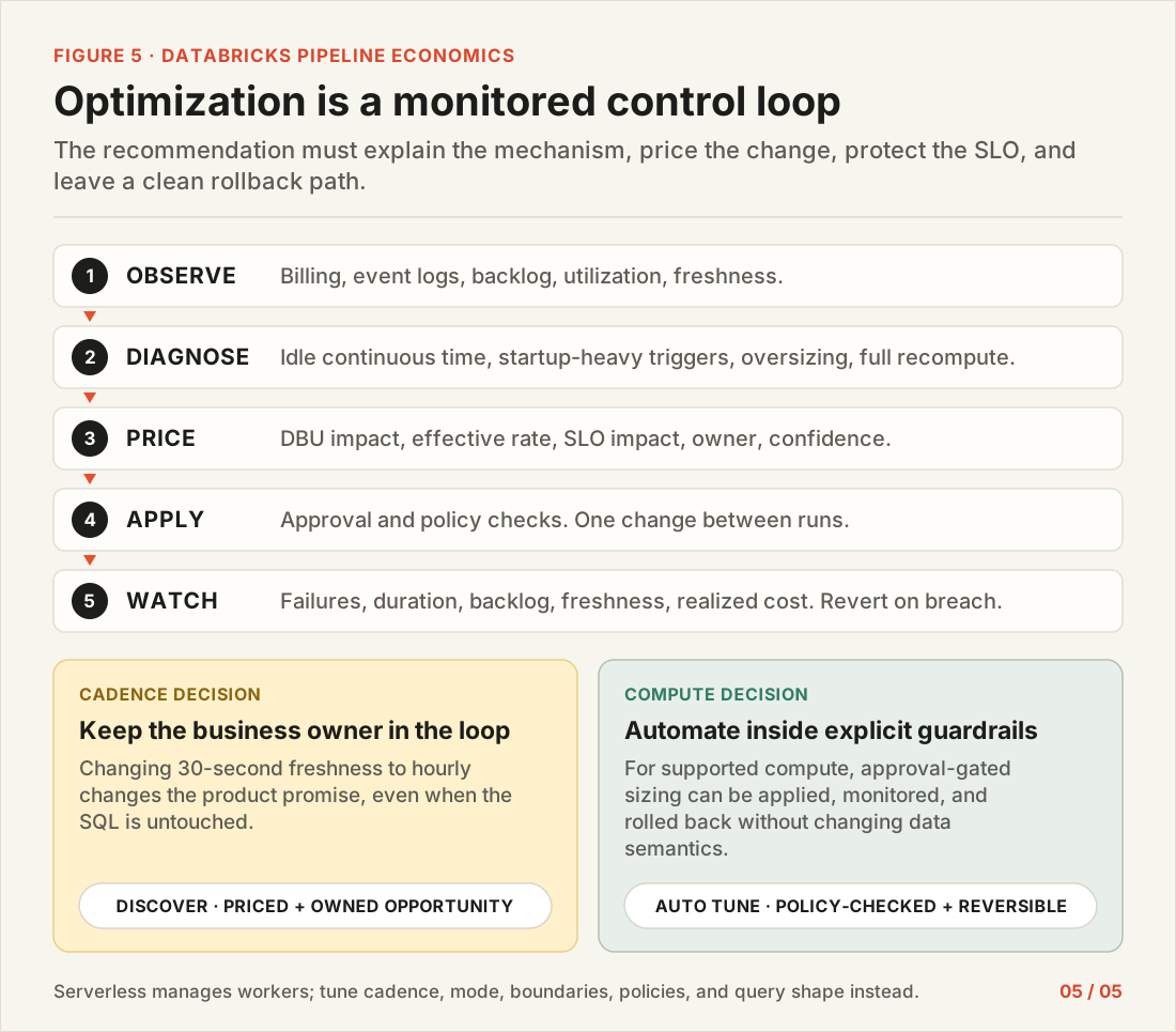
Figure 5. Cadence changes alter a business SLO and should remain explicit. Compute changes can be automated more aggressively when they are approval-gated, monitored, and reversible.
How to choose an execution mode for Databricks streaming tables
The cost of a streaming pipeline follows its latency commitments, especially the commitments nobody has re-examined.
Treat these as four separate design decisions:
Dataset type
Refresh strategy
Execution mode
Compute sizing
Start with triggered execution, and move to continuous execution when a measured freshness requirement needs it. At short scheduling intervals, account for startup overhead, because continuous execution may be the more efficient design. Split pipelines when datasets have different cadence, ownership, scaling, or failure requirements. Measure spend from billing tables, explain it with the event log, and validate every change against end-to-end freshness.
The largest saving may leave the SQL untouched and change only how long the pipeline's compute stays available.
Frequently asked questions
Do Databricks streaming tables need to run continuously?
No. A Databricks streaming table records its progress through checkpoints, so it stays incremental in triggered mode. In triggered mode, the pipeline starts, processes the data available when the update begins, commits its progress, and stops. The next update resumes from that checkpoint.
What is the difference between triggered and continuous pipeline mode?
Triggered mode consumes compute only while an update is running. Continuous mode keeps the pipeline active and processes new data as it arrives, which requires continuously available compute. Databricks guidance places triggered pipelines roughly in the ten-minute-to-daily range and continuous pipelines in the ten-second-to-few-minute range.
How much does a continuous streaming table cost compared with a triggered one?
In this article's illustrative model, a continuous pipeline at 6 DBUs per hour uses 52,560 DBUs a year. An hourly triggered pipeline that runs fifteen minutes per update at 3 DBUs per active hour uses 6,570 DBUs a year, which is 87.5% less. Startup overhead, source volume, autoscaling behavior, retries and update duration will change the result for a real pipeline.
When is continuous mode cheaper than a triggered schedule?
At short intervals, triggered execution repeatedly pays for compute provisioning, runtime initialization, checkpoint recovery, and teardown. In one Databricks employee benchmark, each triggered lifecycle on a five-minute schedule took between 153 and 194 seconds. At sufficient utilization, continuous execution may not be the more expensive design.
How do I find which Lakeflow pipelines run continuously?
In the Databricks system tables, join system.billing.usage, which attributes Lakeflow usage through usage_metadata.dlt_pipeline_id, to system.lakeflow.pipelines, which holds settings such as continuous and serverless. Then inspect system.lakeflow.jobs for CONTINUOUS triggers, because Job orchestration overrides the pipeline's configured mode.
Is a Databricks DLT pipeline the same as Spark Declarative Pipelines?
Yes. In June 2025 Databricks renamed DLT to Spark Declarative Pipelines on Lakeflow, and no migration is required. A Databricks DLT pipeline and a Lakeflow pipeline are the same product, so the execution-mode trade-offs in this article apply to both.