Two recommendations come up in almost every Databricks cost review. First, if a fixed cluster looks underused, reduce the worker count. Second, if demand changes during a run, enable autoscaling. Both sound like easy ways to stop paying for redundant compute.
I had a cluster that seemed to fit the first case. It ran with four Standard_D4ds_v5 workers, but the Metrics tab showed low CPU for much of the job. So I decided to cut it down to two workers, expecting a decent saving. Instead, it made the job 88% slower (363 seconds against 193 seconds) and about 13% pricier in compute.
So I looked at autoscaling, which is the more sensible next step. I configured the cluster to start with one worker and scale to four, expecting it to add capacity for the busy part and reduce it when demand dropped. However, the run took 482 seconds and cost about 75% more compute than the original.
How come two reasonable changes make the same workload slower?
Three runs of the same job show what right-sizing changes, where autoscaling helps, and what to check before you resize a Databricks cluster to cut cost.
Right-sizing and autoscaling change different Databricks cluster settings
Right-sizing covers more than the number of workers. It can include the worker and driver instance types, their sizes, and the number of workers assigned to the cluster. In this post, I kept the instance type fixed at Standard_D4ds_v5 for the workers and the driver and changed only the worker count: four fixed workers in run 1, two fixed workers in run 2, and autoscaling between one and four workers in run 3.
A fixed cluster uses one worker count:
{
  "node_type_id": "Standard_D4ds_v5",
  "num_workers": 4
}
An autoscaling cluster uses a minimum and maximum:
{
  "node_type_id": "Standard_D4ds_v5",
  "autoscale": {
    "min_workers": 1,
    "max_workers": 4
  }
}
Databricks shows the same choice in the compute UI. Without autoscaling, you enter Workers. With autoscaling enabled, you enter Min and Max.
Databricks autoscaling does not choose those numbers for you. It only adds or removes workers within the range you configure. You still need to decide:
whether
max_workersis high enough for the busiest part of the jobwhether
min_workersis high enough for the work that starts before the cluster can scale outwhether the high- and low-demand parts of the job last long enough for scaling to help.
The minimum, maximum, and the length of each workload phase all affect whether Databricks autoscaling helps. The autoscaling cluster I tested in run 3 started at one worker, which shows why.
Three Databricks cluster configurations ran the same job
The workload I described in the opening paragraphs had two phases:
The first phase shuffled and joined the full dataset. It created more parallel work.
The second phase ran 40 short iterations over a narrow slice and needed fewer workers.
I ran the same job on an Azure Databricks workspace with Standard_D4ds_v5 workers. The worker type, driver type, and workload stayed the same. Only the cluster sizing configuration changed.
For a production sizing decision, repeat each configuration several times and compare the median results. The three runs here show how worker count, runtime, and autoscaling timing interacted in this comparison.
Job-time compute cost in the table is node-seconds priced at the Azure pay-as-you-go list rate, explained in the pricing section below.
| Run | Configuration | Runtime | Change from run 1 | Compute cost of one run | Change in cost from run 1 |
|---|---|---|---|---|---|
| 1 | 4 workers | 193 seconds | Baseline | about $0.22 | Baseline |
| 2 | 2 workers | 363 seconds | 88% longer | about $0.25 | 13% more |
| 3 | Autoscaling from 1 to 4 workers | 482 seconds | 150% longer | about $0.38 | 75% more |
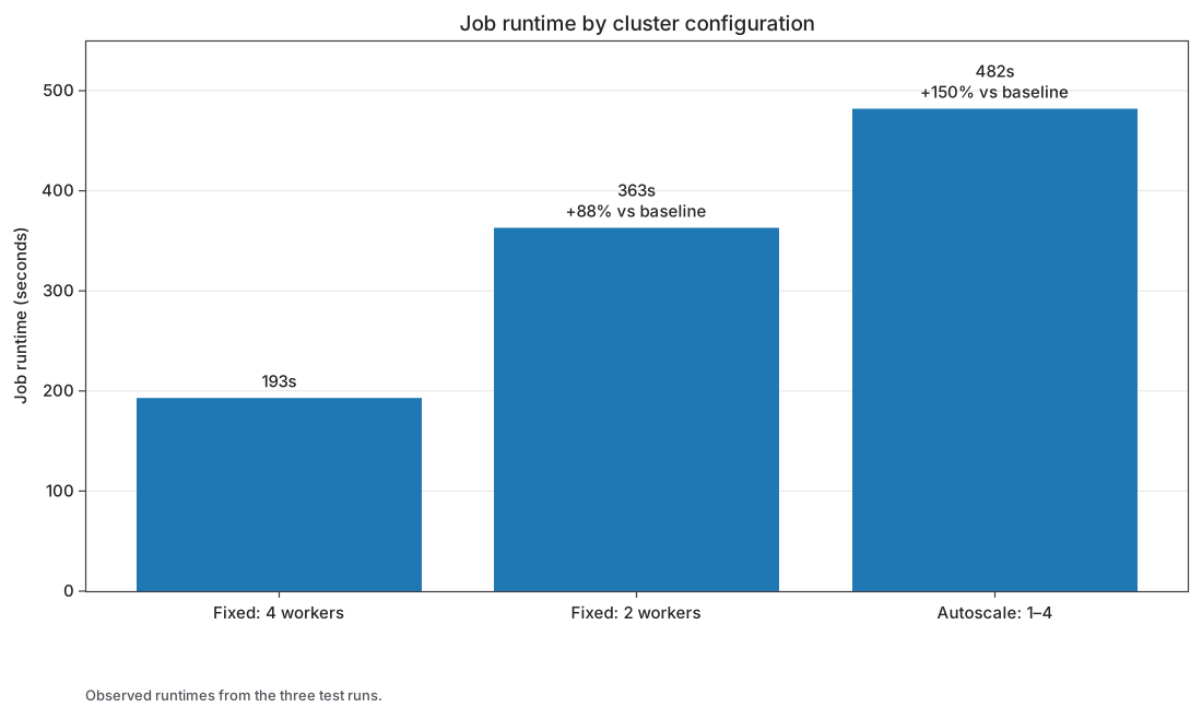
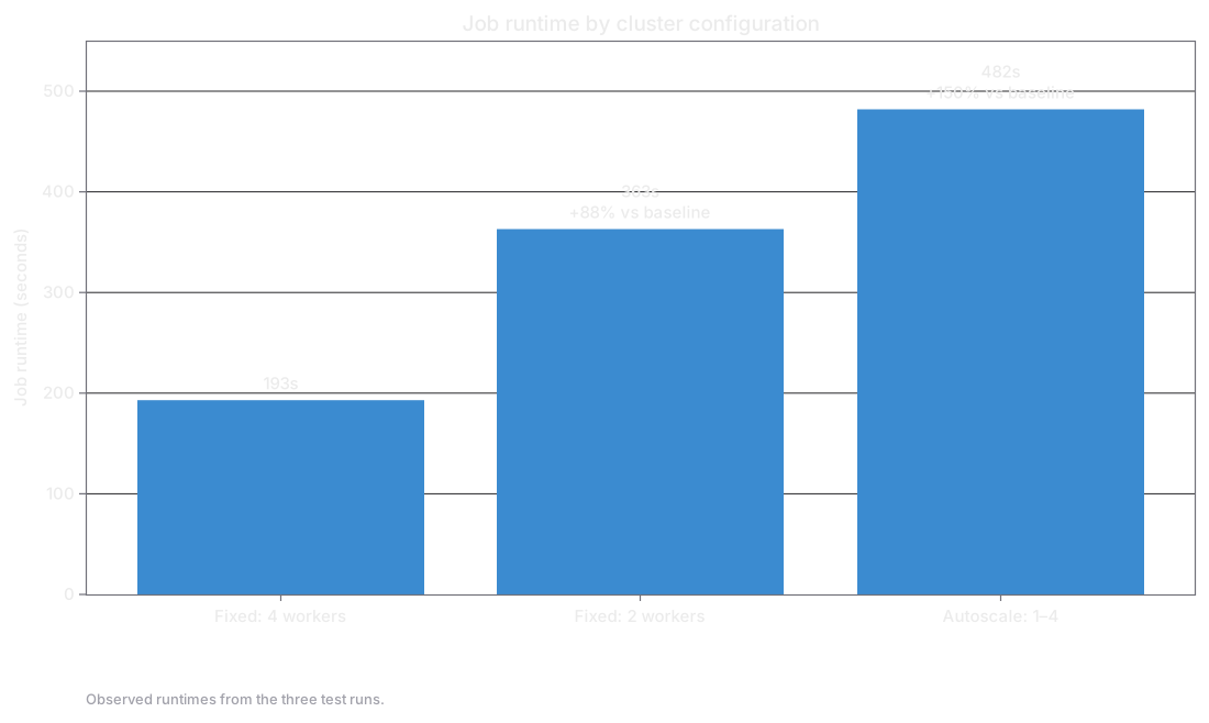
Job runtime for the three Databricks cluster configurations.
Because runs 1 and 2 used fixed worker counts, they have a clear break-even point that we can calculate. Run 3 needs a different comparison: when the additional workers became available and how that timing affected the job.
Run 1 with four fixed workers
Run 1 was the configuration I initially wanted to reduce. It completed the job in 193 seconds. The active-worker line stayed at four while CPU use rose and fell below it.
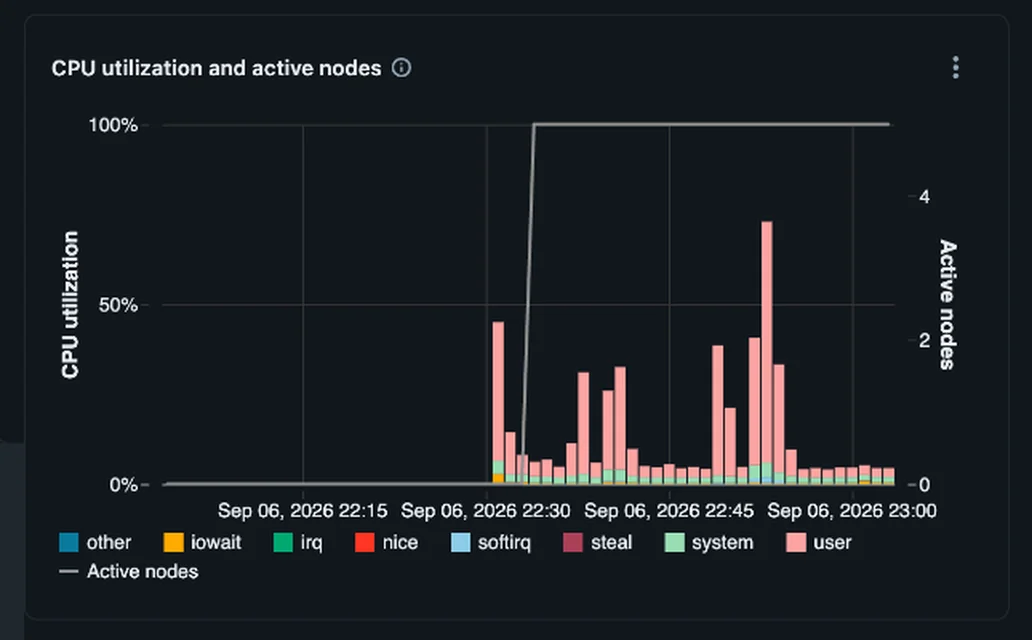
Run 1 CPU utilization and active nodes. Four workers remain active while CPU demand varies.
In the screenshot, the average CPU level makes the cluster look too large. But the metrics chart does not tell us whether tasks were queued during a short peak, whether the job waited on I/O, or whether it used all available parallelism for part of the run.
The Metrics tab is a useful place to find a cluster worth reviewing, but it is not enough to decide the new worker count by itself.
Run 2 with two fixed workers
First, I cut the fixed worker count from four to two. Run 2 took 363 seconds to complete. Including the driver, its Spark node count dropped from five to three.
Because the worker and driver types stayed the same, Spark node-seconds give us a simple way to compare the two fixed configurations.
The baseline used:
5 Spark nodes × 193 seconds = 965 Spark node-seconds
To stay below 965 node-seconds, the three-node configuration had to finish within:
965 ÷ 3 = 321.7 seconds
It took 363 seconds:
3 Spark nodes × 363 seconds = 1,089 Spark node-seconds
The cluster used fewer nodes at any one time, but the longer runtime pushed job-time node-seconds 13% above the baseline.
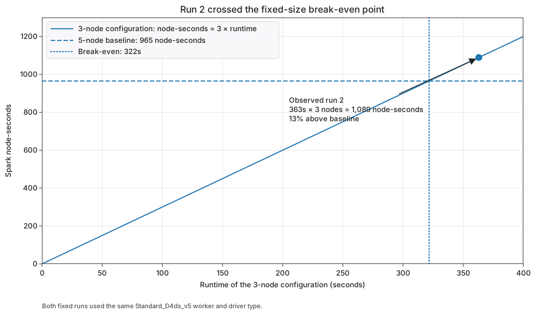
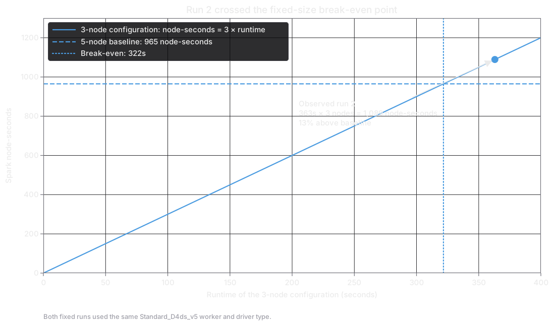
Run 2 crossed the 322-second break-even point for the fixed-size comparison.
The Metrics view confirms that the cluster stayed at two workers:
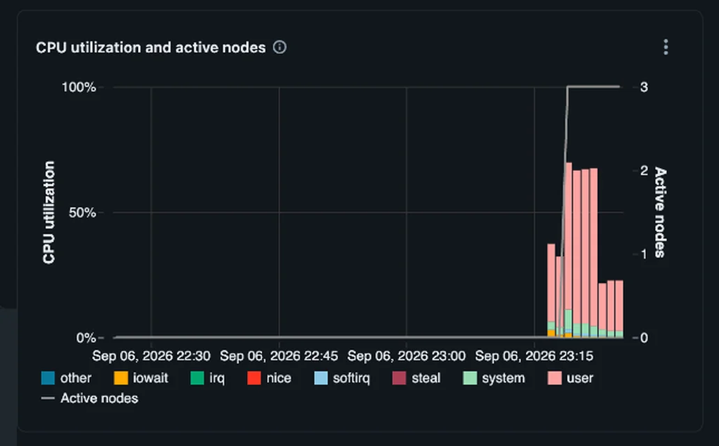
Run 2 CPU utilization and active nodes. Two workers remain active throughout the measured period.
The Spark UI provides the context missing from the average CPU chart. Two executors were available at the start. The shuffle-heavy first phase took most of the runtime, while the 40 short iterations were packed into the smaller block near the end.
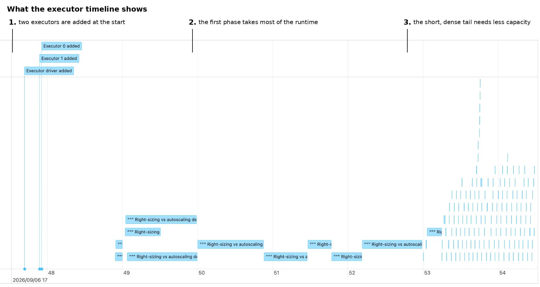
Annotated Spark UI event timeline for run 2.
Two workers were enough for the second phase. They were not enough for the first. The job crossed its 322-second break-even point before it finished.
Run 3 with autoscaling from one to four workers
The third run was meant to maintain access to four workers without using all four for the complete job. I configured autoscaling from one to four workers.
The run completed in 482 seconds, making it the slowest of the three. Run 3 was also the most expensive. Autoscaling changes the node count during the run, so I derived its node-seconds from the measured compute share, which came to about 1,690 node-seconds against 965 for run 1. That is a 75% increase in compute, larger than the 13% increase in run 2.
The Metrics view shows that the worker count increased after the workload had started:
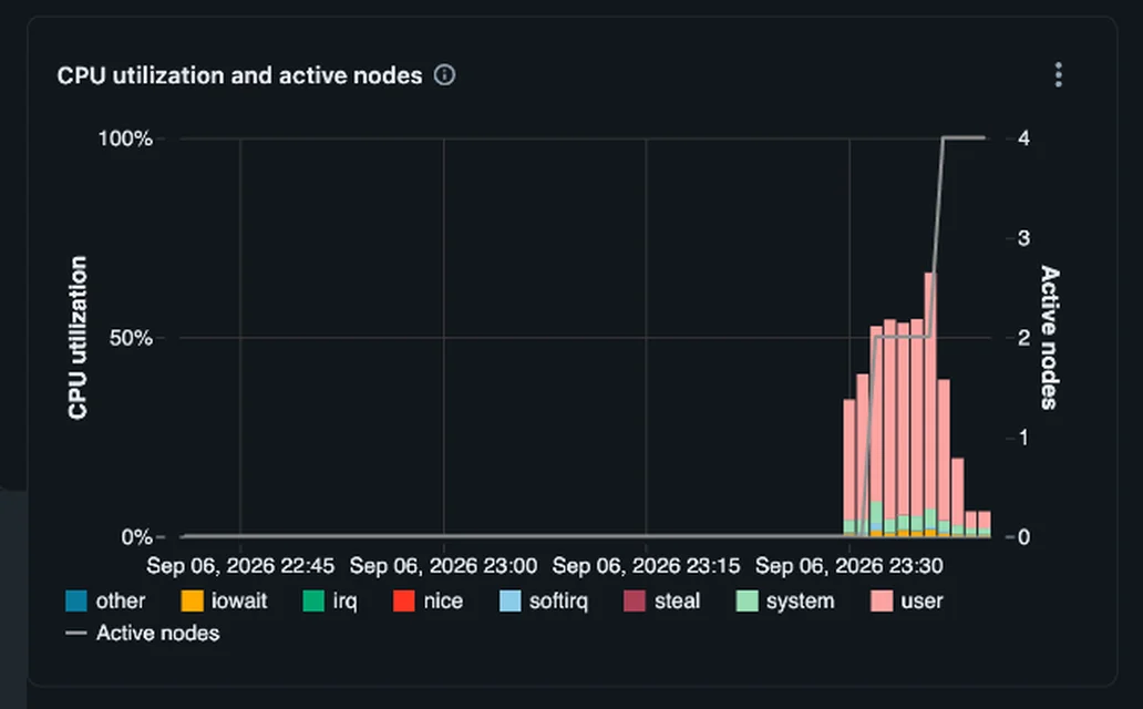
Run 3 CPU utilization and active nodes. The active-worker line rises during the workload.
The Spark UI shows one executor at the beginning, two more arriving at about minute six, and another executor appearing later.
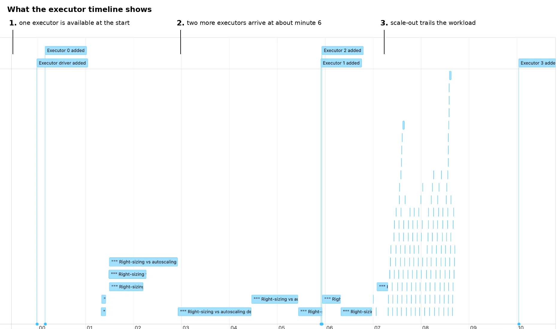
Annotated Spark UI event timeline for run 3.
The autoscaling timing matters in two places. First, an autoscaling cluster starts with min_workers. If the busiest phase begins immediately, setting a low minimum can slow the job while Databricks adds workers. The Databricks compute configuration docs (Azure, AWS) state that optimized autoscaling can move from the minimum to the maximum in at most two scaling events, but the additional workers still need time to become available.
Second, demand must remain low long enough for workers to be removed. On workspaces on the Premium plan, Databricks uses a 40-second underutilization window for job compute and a 150-second window for all-purpose compute. If a lighter phase is shorter than that window, the job may finish before scale-down occurs.
That is what happened in this run. The busiest phase came first, but the cluster started with one worker and added the others after work was already running. The second phase, the 40 short iterations, lasted about a minute, shorter than the 150-second window for all-purpose compute. The 1-to-4 range therefore slowed the first phase and had little opportunity to remove workers during the second.
For this job, min_workers: 1 was too low. A more useful follow-up would compare autoscaling ranges of 2-to-4 and 3-to-4 workers with the fixed four-worker baseline.
Why fewer workers and autoscaling both raised Databricks cost
Reducing the worker count changes two things at the same time. It lowers the amount of compute available per minute, but it can also increase the number of minutes needed to finish the job.
In the fixed-size comparison, the node count fell by 40%, but runtime increased by 88%. The longer runtime was enough to offset the smaller cluster, and job-time node-seconds increased by 13%.
A single run differs by cents, which is why this kind of change passes a review unnoticed. The difference appears when the job repeats. If the same job runs every hour (720 runs a month), the monthly compute cost looks like this:
| Run | Monthly compute cost | Difference from run 1 |
|---|---|---|
| 1: 4 workers | about $158 | Baseline |
| 2: 2 workers | about $178 | about $20 more |
| 3: autoscaling 1 to 4 | about $276 | about $118 more |
These figures are measured across three runs. I multiplied node-seconds by the Azure pay-as-you-go list price for Standard_D4ds_v5 on a Premium workspace ($0.55 for the 1.00 DBU per hour plus the VM). Your negotiated rate and your region will change the dollar amounts. The percentages stay the same.
Databricks autoscaling had a different problem. The maximum still allowed four workers, but the minimum of one did not suit a job that started with its busiest phase. Additional workers arrived after the work had already begun.
The next useful comparison is an autoscaling range such as 2-to-4 or 3-to-4, rather than another lower fixed count, repeated several times and compared with the four-worker baseline.
How to compare Databricks compute cost with node-seconds
The Databricks pricing model depends on the compute product, the amount of compute used, and how long it runs. On classic compute, the cloud provider also charges for the underlying virtual machines and related infrastructure. The exact Databricks cost therefore varies by cloud, region, compute type, plan, and account agreement.
For the two fixed-size runs in this test, the compute type and node types stayed the same. That is why node-seconds are useful for comparing job-time compute:
Spark node-seconds = (number of workers + 1 driver) × runtime
For run 1, that gives 5 nodes × 193 seconds = 965 node-seconds. At $0.816 per node-hour, that is 965 ÷ 3,600 × $0.816, about $0.22. Run 2 is 3 × 363 = 1,089 node-seconds, about $0.25.
This is a comparison method, not an account-specific price. It tells us whether the reduction in nodes was large enough to make up for the increase in runtime.
To calculate Databricks pricing for your own environment, use the usage records in system.billing.usage, apply the relevant list price from system.billing.list_prices, and include the infrastructure charges from your cloud provider where applicable.
The billed cost in system.billing.usage came out lower for runs 2 and 3 than for run 1, because run 1's cluster sat idle for about 36 minutes before I deleted it. That idle time is not part of the job, so I compared job time only.
How to use Databricks metrics and the Spark UI to find sizing candidates
Databricks compute metrics are collected every minute, so a short peak can disappear inside an average. Use the Metrics tab to identify a cluster that may need a sizing change, then check the Spark UI before changing its worker count.
| What you see | What to check next | Change worth testing |
|---|---|---|
| Low CPU, no pending tasks, little spill or garbage collection, and enough runtime headroom | Task concurrency, scheduler delay, I/O wait, and several runs | Reduce the worker count or instance size in small steps. |
| Low CPU with high I/O wait, spill, garbage collection, or driver pressure | Stage metrics and hardware metrics | Fix the resource mismatch or the job before removing workers. |
| Pending tasks or long scheduler delay during a busy phase | Stage timeline and executor saturation | Keep or raise the fixed worker count or max_workers. |
| Long high- and low-demand periods in the same run | Worker timeline and phase duration | Test autoscaling and tune both min_workers and max_workers. |
| Heavy work starts immediately and the cluster scales out later | Executor-add events | Raise min_workers, start with more capacity, or use a fixed cluster. |
A low average CPU line is a reason to investigate a cluster, and on its own it does not tell you the new configuration.
Autoscaling is unavailable or limited for some Databricks workloads
Databricks autoscaling is not available, or does not behave the same way, for every workload.
| Workload or configuration | Databricks behavior | What to do |
|---|---|---|
spark-submit jobs | Databricks documents that autoscaling is not available. | Use fixed sizing for this job type. |
| Structured Streaming on classic compute | Scaling down has limitations. Databricks recommends Lakeflow pipelines with enhanced autoscaling for supported streaming workloads. | Do not assume the cluster will regularly return to a low minimum. |
spark.dynamicAllocation.enabled with Databricks autoscaling | The two systems can make conflicting executor and worker decisions. | Use Databricks autoscaling instead of enabling both. |
Check the workload type before deciding that autoscaling is the next cost optimization step.
AWS Databricks pricing separates DBU and infrastructure charges
The runs in this test were performed on Azure Databricks, but the worker-sizing issue is not specific to Azure. A smaller Databricks cluster on AWS can also lose its expected saving when runtime increases more than the node count decreases.
The final AWS Databricks pricing calculation is different. For non-serverless compute, the Databricks charge and the underlying AWS infrastructure charges are separate. Use the runtime and worker-count comparison in this post to test configurations, then apply the DBU price and AWS infrastructure rates for your own account.
The 13% job-time node-second increase from this Azure test should not be copied directly into an AWS cost estimate. The workload behavior may transfer, but the price does not.
How to choose between right-sizing and autoscaling
Four workers looked underused in the Metrics tab. Reducing the cluster to two workers looked like an easy saving, and autoscaling from one to four looked like the next logical step. Across these three runs, both changes made the job slower (and therefore 13% and 75% more expensive in job-time compute).
The fixed cluster crossed its break-even point because the first phase needed more workers. The autoscaling cluster started that same phase with one worker and added capacity after the work had begun.
For Databricks cost optimization, start with the job rather than the average CPU number. Find when the job needs the most capacity, choose a fixed worker count or autoscaling range that can handle it, and then compare the result with the original run.
Give the job enough capacity for its busiest phase, without keeping workers it does not need.
Frequently asked questions
Does Databricks autoscaling reduce cost?
Not always. In this test, autoscaling from one to four workers took 482 seconds against 193 seconds for four fixed workers, and cost about 75% more in job-time compute. The cluster started its busiest phase with one worker and added workers after the work had begun.
What is the difference between right-sizing and autoscaling in Databricks?
Right-sizing can change the worker and driver instance types, their sizes, and the number of workers assigned to the cluster. Databricks autoscaling only adds or removes workers within the min_workers and max_workers range you configure, and it does not choose those numbers for you.
Why did cutting a Databricks cluster from four workers to two cost more?
The node count fell by 40%, but runtime increased by 88%, from 193 to 363 seconds. Job-time node-seconds rose from 965 to 1,089, which is 13% above the four-worker baseline.
How long does Databricks wait before autoscaling removes workers?
On workspaces on the Premium plan, Databricks uses a 40-second underutilization window for job compute and a 150-second window for all-purpose compute. If a lighter phase is shorter than that window, the job may finish before scale-down occurs.