Authors and Databricks itself publish many guides on Databricks cost optimization. They cover techniques, strategies, approaches, and what to do and not do. The guides converge on the same checklist: turn on auto-termination, use job clusters, try spot instances, enable Photon...
None of that is wrong. The problem is that it assumes you already know where your money is going, and most teams don't.
We still need to make sense of how Databricks compute actually works. What decides your Databricks bill when you get billed for the usage in a month? It sounds easier to just say, "Hey, you’ve used 300 DBU. The DBU rate is $0.40 per DBU. That means 300 DBU times $0.40 = $120, right?"
But then you might be wondering about that DBU 300; is that the only cost you need to take into account? What did it cost to keep the compute running that consumed those DBUs? And if someone asked you what the marketing team's dashboards cost last month, or how much of that was compute sitting idle, could you answer?
How Databricks DBU Cost and Cloud Infrastructure Cost Add Up
The Lakehouse model stores data once in open formats and brings compute engines to that data, instead of copying it into a separate warehouse for analysis. That is one of the core economic principles behind the Databricks model.
To understand how this affects your Databricks billing, see how Databricks decouples three core layers:
Storage: Holds the data indefinitely in open formats at raw cloud storage rates.
Governance: Controls access and security across the entire data estate via Unity Catalog.
Compute: Executes work against the stored data on demand.
The Databricks Compute layer
Databricks compute is the execution layer. It is where queries run, notebooks execute, jobs transform data, and machine learning workflows consume governed datasets and turn them into outputs. In the Databricks operating model, storage preserves data and governance defines who can use it, but compute is where value is actually created.
Databricks Compute types
Databricks offers three types of compute:
Serverless Compute: Fully managed compute that is available instantly. Databricks handles cluster provisioning, scaling, and maintenance.
Classic Compute: Compute clusters provisioned directly in your cloud account, giving you full control over node types and configurations.
SQL Warehouses: Specialized compute optimized specifically for SQL queries, BI dashboards, and data warehousing workloads.
Separating storage and compute does not remove their costs. The costs become visible, more distributed, and more operational. So the total Databricks cost becomes a two-bill problem.
The first bill is platform cost, where you pay for the Databricks platform in DBUs.
A DBU, or Databricks Unit, is Databricks’ billing unit for compute consumption. A DBU measures compute power consumed over time. Databricks tracks your bill by compute SKU, usage type, and workload category instead of a single flat "cluster cost". For example, in mid-2026 an all-purpose compute cluster typically costs around $0.55 per DBU-hour for a standard runtime.
The second bill comes from your cloud provider. That bill covers the infrastructure cost: virtual machines, disks, and associated network costs. Serverless compute is the one major exception. Its Databricks DBU charge already includes the virtual machine cost, because Databricks manages that compute itself.
Now go back to the $120 calculation from the intro. That $120 is not the total cost. DBUs are only the Databricks half. The EC2 or VM hours, the disks, the NAT gateway, and the cross-zone traffic arrive on a separate invoice. You don’t see that invoice on the Databricks console. This split is why two common cost conversations go sideways:
A team cuts its Databricks DBU cost by 20% and wonders why the total bill barely moved. The infrastructure half didn't change.
A team compares the serverless DBU rate against the classic DBU rate and concludes serverless costs several times more. But serverless includes the VM whereas Classic doesn't.
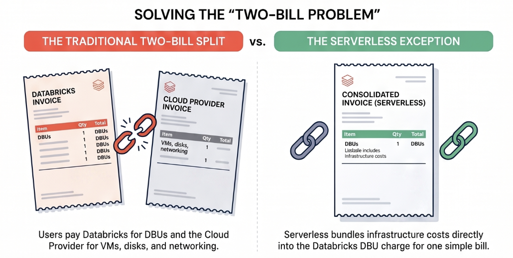
Your Databricks DBU cost covers only half of what you pay. The other half is the infrastructure you kept running to consume those DBUs.
Start With Databricks System Tables and Know Their Gaps
To understand usages, Databricks system tables are the right place to start, and most teams underuse them. Four tables matter most for compute cost, plus one more if you run SQL warehouses:
| Table | What it gives you |
|---|---|
system.billing.usage |
DBU quantities, SKU names, and a usage_metadata struct with cluster_id, warehouse_id, job_id, and job_run_id, plus custom tags and the identity that ran the workload |
system.billing.list_prices |
List prices per SKU over time, so you can turn DBUs into dollars |
system.compute.clusters |
Cluster configuration history, so you see what a cluster looked like when it ran |
system.compute.node_timeline |
Per-minute CPU and memory per node. |
Add system.query.history if you run SQL warehouses, because it records how long queries spent waiting for compute.
To see Databricks DBU cost in dollars, join system.billing.usage to system.billing.list_prices on the SKU name and the period each price was in effect. This query is adapted from the Databricks billing sample queries and returns usage and list cost per SKU for the last 30 days:
SELECT usage.sku_name,
       usage.usage_unit,
       SUM(usage.usage_quantity) AS quantity,
       SUM(usage.usage_quantity * list_prices.pricing.effective_list.default) AS list_cost
FROM system.billing.usage
JOIN system.billing.list_prices
  ON list_prices.sku_name = usage.sku_name
WHERE usage.usage_end_time >= list_prices.price_start_time
  AND (list_prices.price_end_time IS NULL OR usage.usage_end_time < list_prices.price_end_time)
  AND usage.usage_date >= current_date() - INTERVAL 30 DAYS
GROUP BY usage.sku_name, usage.usage_unit
ORDER BY list_cost DESC;
The result uses list prices and does not reflect any negotiated discount.
Before writing anything custom, you can import Databricks' Lakeflow observability dashboard. It ships as JSON you drop into your workspace, and the page publishes the SQL behind every tile.
Note - if you use the Lakeflow observability dashboard, be aware that usage_metadata.job_id is only populated for jobs on job compute or serverless. So filtering billing usage for an all-purpose SKU where job_id is not null returns nothing at all. The empty result only means the filter never had rows to match. To actually find jobs running on all-purpose clusters, you have to go through job_task_run_timeline joined against compute.clusters, and Databricks publishes that query.
None of these Databricks system tables contains a single dollar of cloud infrastructure cost. To get a total bill, you join Databricks usage against your cloud provider's cost and usage report based on resource tags. Databricks does propagate cluster tags.
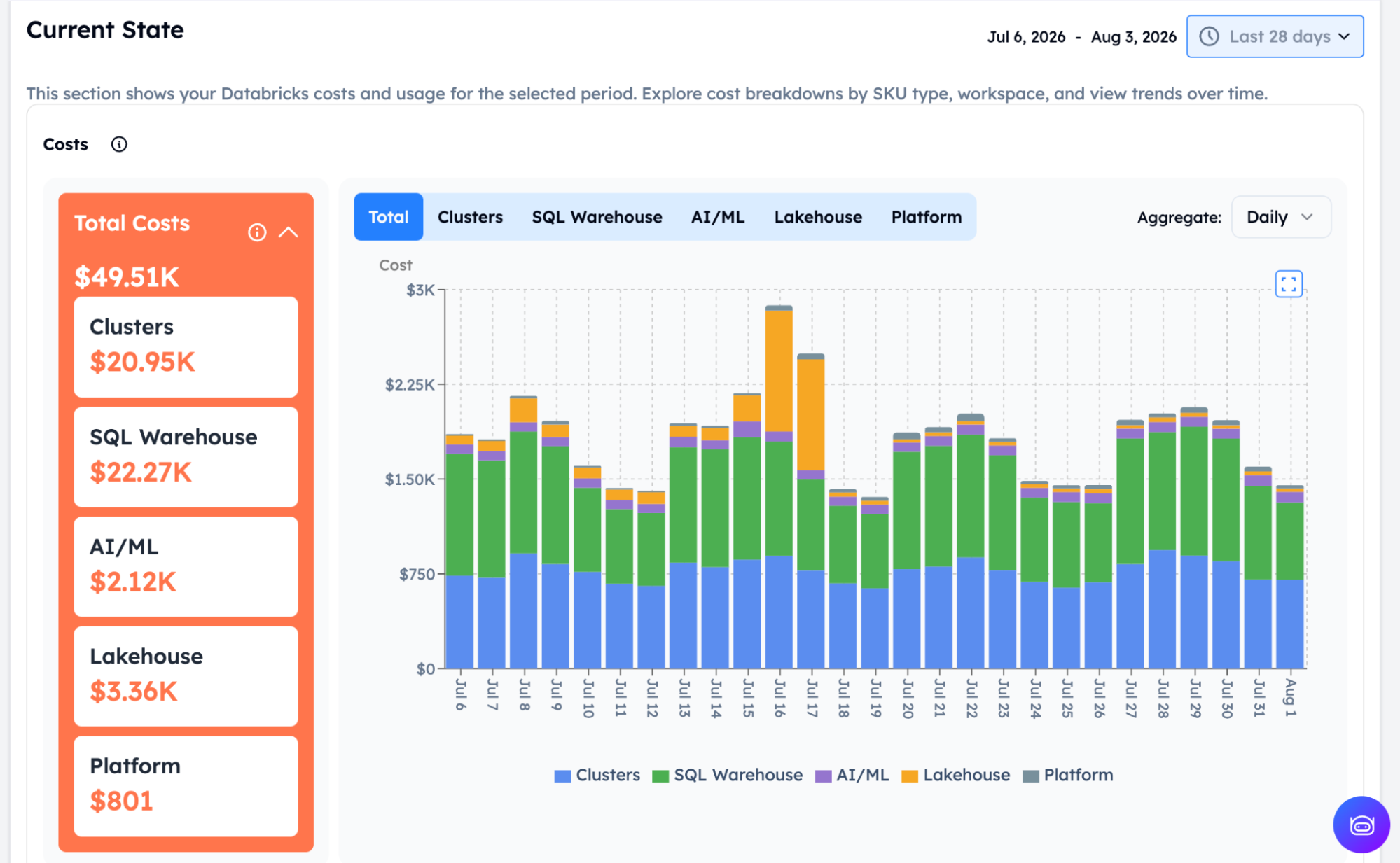
Altimate's Clusters and SQL Warehouses views stitch both halves together and attribute the result down to cluster, warehouse, job, and team. You can read one number per workload instead of reconciling two exports by hand.
Where your compute money goes
Once you start thinking in terms of two bills, the next step is understanding what usually drives the cost. For most teams, Databricks DBU cost and cloud cost go into a familiar set of buckets:
| Where the money goes | Which bill it contributes to | What to look at first |
|---|---|---|
| Idle time on interactive compute | Both | Cluster uptime against query time |
| The wrong compute type for the workload | Databricks (DBU) | All-purpose SKUs running scheduled jobs |
| Oversizing | Both | Node utilization in system.compute.node_timeline |
| Loose or poorly bounded autoscaling | Both | The minimum you always pay, and how long max is held |
| Long-running interactive resources that nobody turns off | Both | Auto-termination settings |
| Streaming patterns that run 24*7 when the business requirement does not actually need 24*7 freshness | Both | Trigger mode against the business requirement |
| Infrastructure side effects such as networking, egress, or duplicated data movement | Cloud only | Your cloud cost and usage report, by tag |
Workloads drift, so revisit the table above on a regular schedule, not only after a bill shock prompts a one-time sprint.
Despite all the efforts, a pipeline can be on the wrong SKU, oversized, and idle half the time, all at once. That pipeline will look completely healthy on every alert you have unless you have visibility at that granular level.
When Serverless Helps, and When It Doesn't
As we discussed earlier, serverless compute is good for bursty workloads such as BI. BI workloads often come in bursts. A user refreshes a dashboard, runs a query, inspects results, then goes idle. In non-serverless warehouses, startup time is long enough that teams often leave resources running to avoid waiting. Serverless can help change this trade-off because it can start and scales in seconds and can terminate idle compute sooner than all-purpose/classic compute.
What you give up is control. No picking instance families, no spot strategy, no pool tuning. That's fine when your problem is startup delay and idle waste. It hurts when your problem needs precise control over the infrastructure underneath the workload.
So skip "is serverless cheaper?" and ask what kind of waste we are trying to eliminate. Serverless is often the best choice at its premium price when the waste comes from slow startups, bursty access, and long idle windows.
Classic compute can cost less when the workload is steady, predictable, and suited to deliberate sizing and cloud cost engineering. That is especially true when teams know their workload shape well enough to right-size aggressively. Those teams can also use cloud primitives that serverless does not expose in the same way.
This is also why visibility comes before optimization. Without data on burstiness, concurrency, and idle windows, the serverless debate turns ideological instead of operational.
Idle and the Wrong Compute Type
These two problems compound each other. Take a big all-purpose cluster. The work finishes fast because the instance is large. But the cluster hangs around afterward because spinning it back up is slow. You're paying double: a costlier instance, and longer idle time on top of it. All-purpose clusters are also much easier to leave running between interactions. Job compute only runs while there's a job to run.
"Job compute is typically 2-3x cheaper than all-purpose," says Databricks’ cost maturity post. Treat that figure as a starting range, not a rule. What you save depends on how much runtime was idle and which half of the bill dominates for that workload. Teams miss this constantly, and the pattern is always the same:
A notebook starts on an all-purpose cluster because development is interactive.
The workflow proves useful.
It becomes production-critical.
Nobody revisits the compute type.
The company pays a production bill for a development pattern.
A quick fix is auto-termination on all interactive compute resources. Add scheduled restart patterns for business-hour usage where startup delay matters. Auto-termination controls idle waste. It does not fix the underlying pattern when the workload lives on the wrong compute type.
It is one thing to tell every team to use job compute. It is more useful to know exactly which production pipelines still run on all-purpose clusters. You also want to know how long those clusters sit idle and what the cost delta looks like. The system.billing.usage and compute.node_timeline join from the previous section answers those questions.
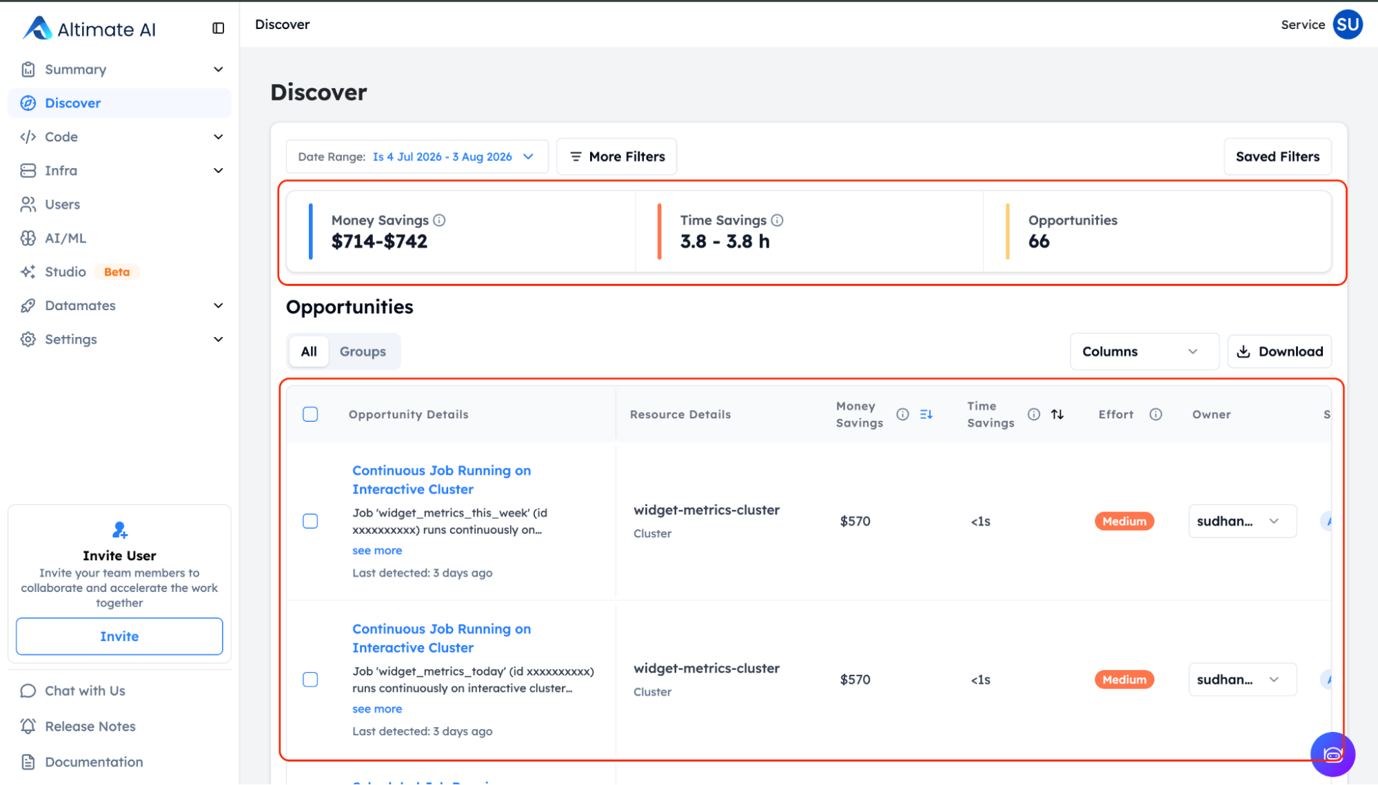
The Discover page in the Altimate.ai enterprise platform surfaces this kind of opportunity.
In the screenshot, Discover flags a continuous job running on an interactive cluster and suggests switching it to a serverless job or a job cluster. Read more about Databricks cost optimization with Altimate.
Spot and Fleet Instances
On classic compute, spot is still the most underused lever. Use spot instances for workloads that can tolerate interruptions. Keep the Spark driver, which is the first instance, on demand. Run the workers on spot capacity. Keep the Fleet instance types on AWS, where Databricks can choose the best-matching physical instance types by price and availability. See more in Databricks' guidance on choosing optimal resources.
However, Spot is not a universal answer. It works best when the workload is fault-tolerant and when retry, checkpointing, or restart behavior makes interruption acceptable. Batch ETL, retry-friendly pipelines, and some model-training jobs are natural candidates. Low-latency or interruption-sensitive workloads are not.
Spot only touches the cloud bill. It does nothing to reduce Databricks DBU consumption. So on Jobs Compute, where the DBU rate is low and infrastructure is a large share, Spot moves more of the bill. On All-Purpose, where DBUs dominate, fixing the SKU matters more. Know which half you are attacking before you pick the lever.
Levers like these are why classic can still beat serverless on cost for stable workloads, and why it demands more operational maturity. Someone has to decide what's interruption-tolerant, enforce the driver/worker pattern, and keep it consistent.
The cheapest Databricks configuration is usually the one whose behavior matches the workload, not the one with the lowest nominal unit rate. It also helps to know which levers that configuration actually exposes.
Autoscaling That Doesn't Behave How You'd Expect
Most people picture autoscaling as something that tracks CPU. Databricks autoscaling does not track CPU. Databricks describes its optimized autoscaling in terms of workload behavior. Worker allocation reacts to job characteristics, mainly the backlog of pending tasks.
A cluster can scale up while its existing nodes sit at 30 percent CPU because the stage produced a lot of small tasks. It can also stay flat under heavy CPU load because the work is never split into enough tasks to create a backlog.
Which leads to five things people get wrong:
A wide min/max range is not free insurance. If you set the range to 2 to 20, a burst of small tasks pulls you toward 20. Autoscaling holds those nodes for the stage and bills you. Autoscaling did its job. The range was the decision, and the range was a guess.
Your minimum is a floor you always pay. A minimum of 8 workers means you never pay for fewer than 8, including the long tail where one straggler task is finishing.
Streaming does not scale back down the way batch does. A continuous stream always has work in flight. So the underutilization condition rarely holds. Databricks recommends Lakeflow pipelines with enhanced autoscaling for streaming rather than treating standard autoscaling as universal. Databricks also recommends triggered incremental patterns like AvailableNow when the business does not need 24/7 freshness. Whether you need 24/7 freshness is usually the bigger cost question.
Autoscaling does not fix oversizing. It is a range. Give it the wrong range, and it arrives at a wrong number faster.
Cluster autoscaling and SQL warehouse scaling are not the same system. Conflating the two is expensive, and it is worth its own explanation below.
Warehouse size and warehouse scaling are different dials
A SQL warehouse has two independent settings:
Size (2X-Small up to 4X-Large) is how much compute sits behind one cluster. Each step up doubles the worker count, from 1 worker at 2X-Small to 256 at 4X-Large, and the DBU rate scales with it. A bigger size makes a single heavy query faster.
Scaling (min and max clusters) is how many identical clusters sit behind the warehouse. More clusters means more queries run at once. It does nothing for the speed of any single query.
To understand, let’s take an example: users say the warehouse is slow. Someone bumps the size, which doubles the rate. But the actual problem was 30 analysts hitting it at 9am and queueing. No query was compute-starved; they were waiting. The size increase does not help, so someone bumps it again. You are now paying four times the original rate for a concurrency problem that more clusters would have fixed at the original size.
The diagnostic is queue time in system.query.history. Significant time waiting for compute usually means scaling out, and long execution with negligible queue time means scaling up. Databricks treats a consistently non-zero queue as a sign that you need either a larger size or more clusters. Check which of the two the queue points to before you turn a dial.
How to Right-Size Clusters and Warehouses
"Right-sizing" is the most overused and underexplained phrase in Databricks cost conversations. Databricks' cost optimization best practices explain it as:
Sizing in terms of workload demands: total executor cores, total executor memory, local storage, data partitioning, computational complexity, and parallelism needs. It also recommends starting SQL warehouses at smaller sizes and scaling up only as concurrency and query complexity justify it.
That definition splits right-sizing into several separate questions:
Is this workload interactive SQL, scheduled ETL, ad hoc exploration, streaming, or ML?
Is it on the right compute type at all?
Is the instance family aligned with CPU, memory, shuffle, or caching needs?
Is the driver/worker balance sensible?
Is the warehouse or cluster too large for its actual concurrency pattern?
Is it too small, forcing longer runtime and creating false savings?
Many teams make expensive mistakes because they treat right-sizing as downsizing.
But downsizing is only one possible outcome. Right-sizing can mean moving smaller or moving to a different instance family. It can mean moving a workload from all-purpose to job compute, or a bursty workload to serverless. It can also mean accepting a slightly larger resource, because the shorter runtime lowers the total cost.
This distinction becomes more important in mixed Databricks environments where SQL warehouses, Spark jobs, development notebooks, and streaming pipelines all coexist. A team that applies one universal sizing philosophy across all of them usually ends up mis-sizing most of them.
How to pick a right family instance for jobs
Instance-family choices are a bit of a cumbersome decision but the highest-impact compute decisions in Databricks cost optimization.
Databricks gives some simple rules of thumb in its AWS guidance:
memory-optimized for ML, heavy shuffle, and spill-heavy workloads
compute-optimized for structured streaming and maintenance jobs
storage-optimized for workloads that benefit from caching, such as ad hoc or interactive analysis
general-purpose when there is no specific dominant requirement
GPU only where GPU-accelerated libraries actually justify it, per Databricks’ cost optimization best practices
The same rules apply to the other cloud providers. Instance family is a cost decision as much as a performance one. A badly matched family can create waste even when the cluster size looks reasonable.
A memory-heavy job on compute-optimized nodes may spill and run longer than necessary.
A shuffle-heavy workload on the wrong family may look “cheap” per node but cost more overall because of runtime inefficiency.
A cached interactive workload on the wrong shape can waste both time and money.
To understand Databricks compute costs, count the nodes. Then ask what kind they are and whether they match your workload pattern.
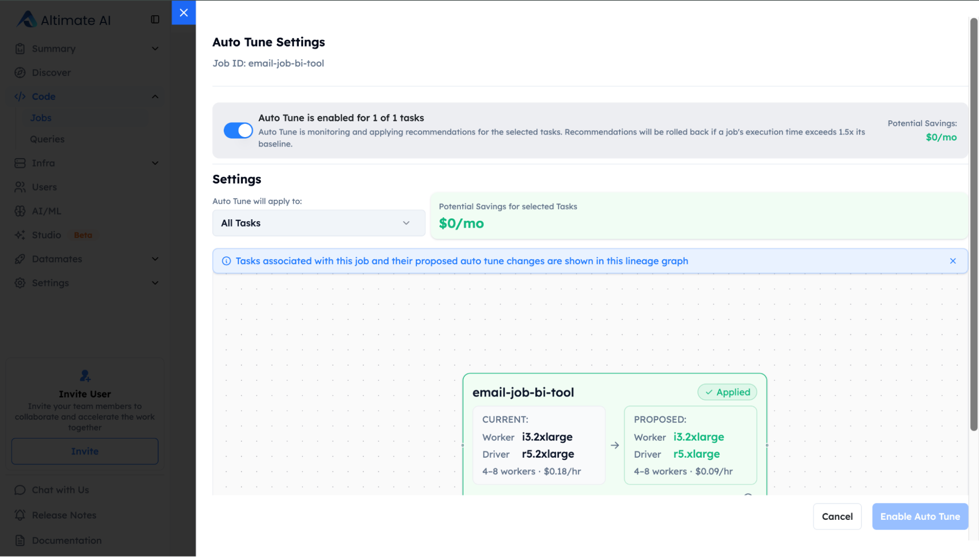
Altimate Auto Tune uses workload behavior to determine if the current compute family is optimal for the workload. Auto Tune shows how your current configuration and our suggested one each perform. You understand the issue before you trust Altimate’s recommendation to make a change.
Keeping compute right-sized over time
You now know what to set: the instance family, the compute type, and the autoscale range. You set all three on the cluster when you create it. Those values can go out of date within a few months, because of
Concurrency changes
Query patterns change.
Teams change. A development environment becomes shared production infrastructure.
A job that used to be small becomes a major pipeline.
A warehouse sized for one dashboard becomes the default for ten.
Right-sizing is an ongoing process. Databricks recommends regular cost audits, ongoing monitoring, tagging, budgets, dashboards, and revisiting strategies as environments scale or change. This is also where operator (FinOps) trust becomes part of the conversation.
As soon as you move from we should size better to a system should help us keep sizing current, the obvious questions appear:
How much access does the system need?
What is the blast radius if it gets something wrong?
Is there an approval step?
Is there an audit trail?
Can I dry-run it first?
Can it roll back?
What does rollback restore, and what does it not restore?
Rollback restores configuration. It does not restore time. If a change made a pipeline late, rollback fixes the next run. But the data that landed late stays late, and downstream jobs already read it as stale.
How Altimate Auto Tune adds control

The rollback limit is why Auto Tune leans on scope, verification, and rollback instead of asking you to trust it. Auto Tune is two agents, one for jobs and one for SQL warehouses. Each agent gets its own guardrails.
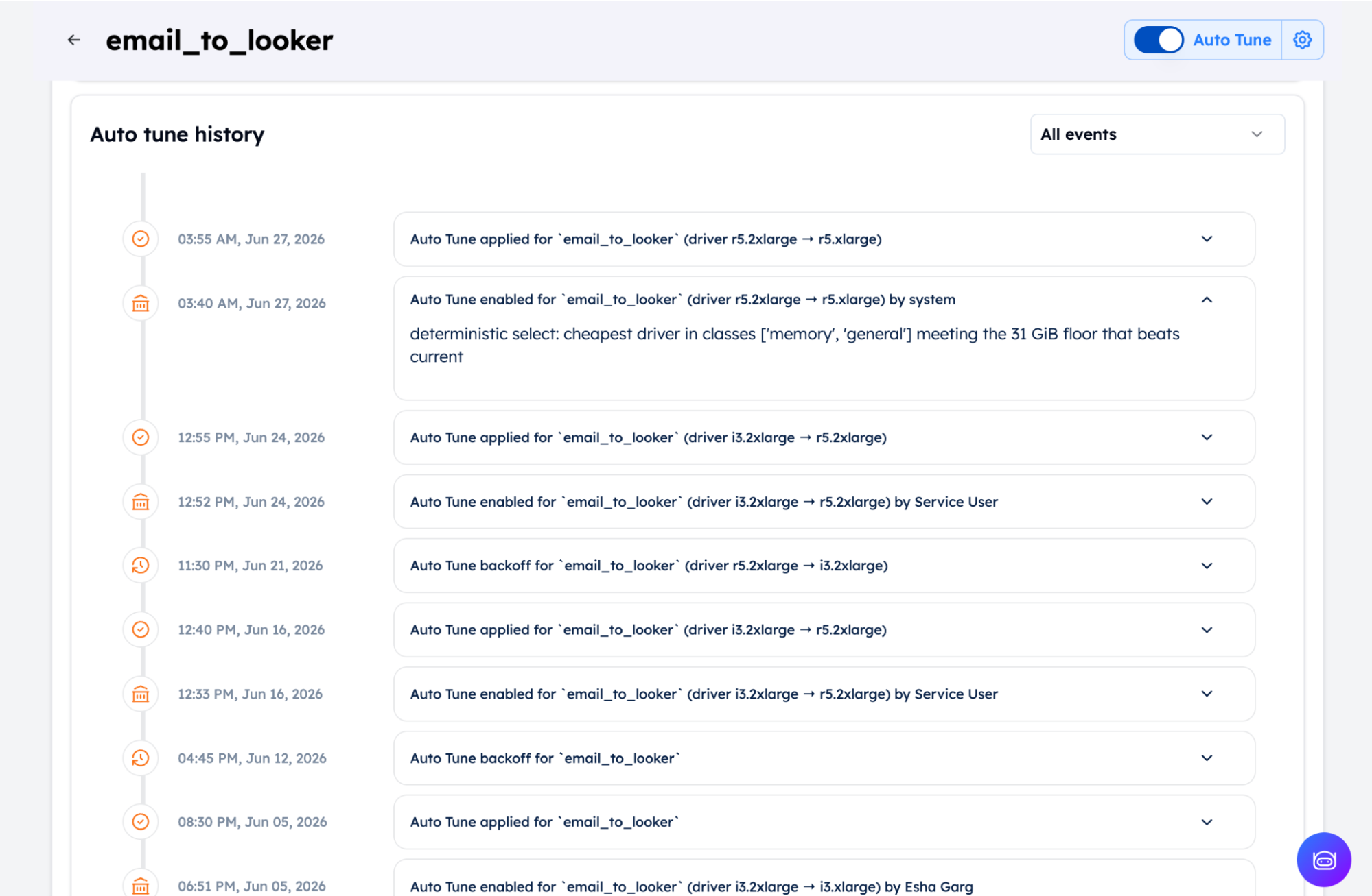
Snapshot, apply, verify: Every change captures the original config and applies the update. Then Auto Tune reads the config back to confirm the change took. The original is always exactly restorable.
Performance monitoring with automatic backoff: Auto Tune watches performance against the recent baseline after every change. It tracks latency for warehouses and run health for jobs, and rolls back automatically if something regresses.
Granular and approval-gated: Control is per job, per task, and per warehouse. Nothing changes until you enable a recommendation. Jobs only change while idle and after policy checks pass.
Stays current: Once enabled, Auto Tune keeps following newer recommendations as the workload changes, under the same monitoring and backoff. That is how sizing stays current instead of going stale by next quarter.
Fully audited: Auto Tune timestamps every requested, applied, failed, and backoff event with who, which job or task, before, and after. You can filter and export those events.
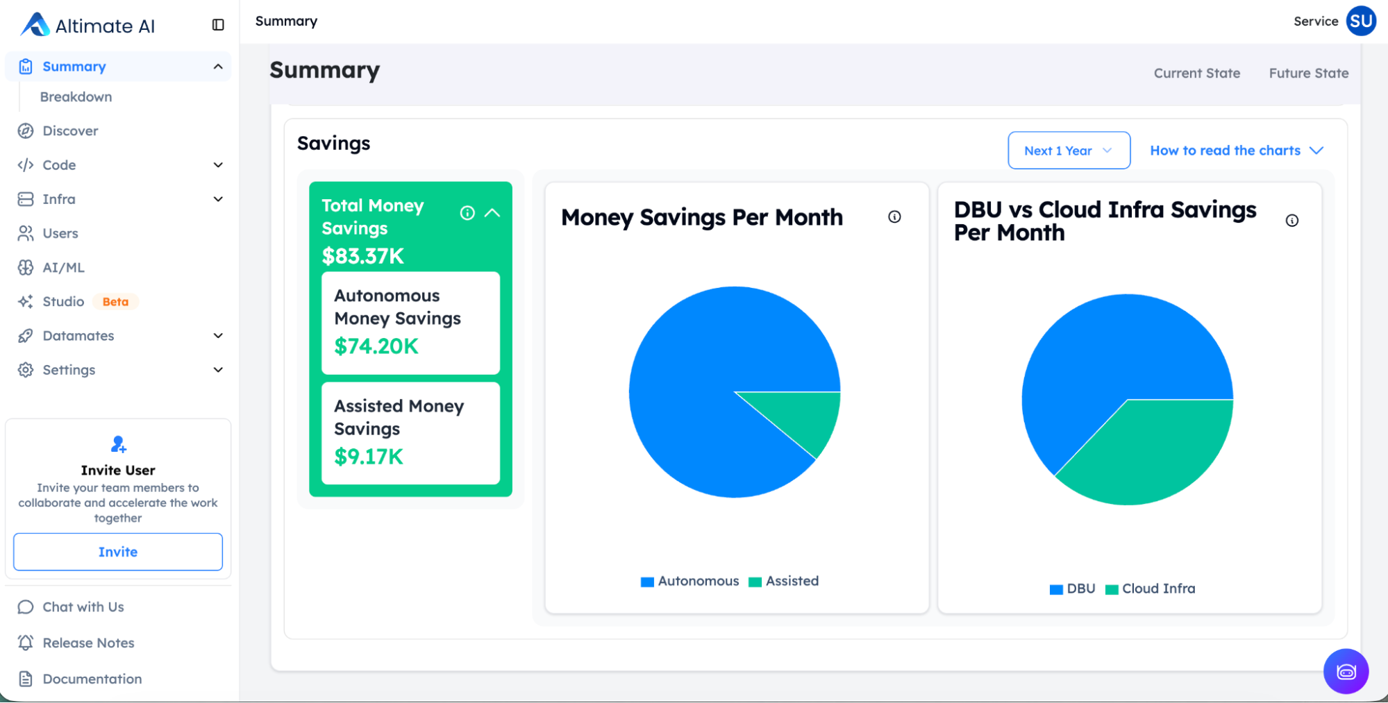
Savings you can see: Altimate reports realized savings, money already banked, separately from potential savings. Potential savings are ones Altimate identified but did not capture yet. The Autonomous Savings summary page shows the savings, with a breakdown per job and per warehouse if you want to drill down.
Which Compute Type for Which Workload
| Workload | Compute | Key settings |
|---|---|---|
| Interactive BI | Serverless SQL warehouse | Right-size, short auto-stop, scale out on concurrency |
| Ad hoc SQL and exploration | Serverless, or classic with tight auto-termination | Start smaller than feels comfortable, size up on evidence |
| Scheduled ETL and batch | Job compute plus Auto Tune | On-demand driver, spot or fleet workers, narrow autoscale range |
| Short frequent jobs | Serverless jobs, or classic with a pool | Measure startup as a share of total runtime first |
| Streaming | Job compute, or Lakeflow with enhanced autoscaling | Evaluate triggered (AvailableNow) before assuming always-on |
| ML training | All-purpose or job compute with GPU | Pools for iteration, right-sized driver |
The cheapest option depends on the workload. Compute gets expensive when teams pick one out of habit.
What to Measure Before You Optimize Databricks Compute
On classic compute, your Databricks DBU cost and your cloud infrastructure cost arrive on separate invoices. Read both before you change a setting. Use the Databricks system tables to find which workloads run on which compute type and which clusters sit idle. Most waste comes from idle time, the wrong compute type, and defaults nobody revisited. Join that data to your cloud cost and usage report to measure what spot, autoscaling, auto-termination, and instance-family changes save.
See the official Databricks cost optimization best practices and the well-known cost maturity journey post on the Databricks blog.
Frequently Asked Questions
How Is Databricks DBU Cost Calculated?
Your Databricks DBU cost is the DBUs a workload consumes multiplied by the rate for its compute SKU. An all-purpose compute cluster on a standard runtime costs around $0.55 per DBU-hour in mid-2026. Classic compute adds a separate cloud invoice for VMs, disks, and networking. Serverless compute includes the VM cost in the DBU rate.
How Do You Reduce Databricks DBU Consumption?
Idle interactive compute, oversized clusters, and loose autoscaling ranges all waste DBUs. To reduce Databricks DBU consumption, tighten auto-termination and narrow the autoscale range. Check per-node CPU and memory in system.compute.node_timeline to find oversized clusters. Moving scheduled jobs from all-purpose to job compute lowers the DBU rate. Databricks says job compute is typically 2 to 3x cheaper. Your saving depends on idle time and on which half of the bill dominates.
Do Databricks System Tables Show the Full Compute Bill?
The Databricks system tables hold DBU usage and list prices, but none of them contains cloud infrastructure cost. To get the total bill, join Databricks usage to the cost and usage report from your cloud provider on resource tags.