
The official Databricks price calculator provides you information on the DBU rate times the hours you plan to run, the instance type for cloud providers, the costing of VMs (basically compute types) for the kind of workloads you want to run, and other basic details such as compute options available.
But the cost calculator provides no guidance on the different configurations and parameters that actually affect your overall costs and how to set these.
For instance, it doesn't tell you if you're paying for compute hours you didn't need, running on a compute type that charges more for identical work, or still sized for a large but outdated workload that shrank a quarter ago.
In this blog post, we will cover the six main levers that can help you reduce the cost and help you make better usage decisions. To gain a deeper understanding of how Databricks compute costs work, you should read our Understanding Databricks Compute Cost post, which will clarify the total cost of running Databricks, including cloud infrastructure and workload pricing (i.e., per DBU).
Let’s start with a very common yet underused cost lever. The few people who do use this lever often don’t use it in an optimal way.
Cost Lever #1: Match Compute Type to Workload Before Anything Else
Before selecting your Databricks compute type, analyze your workload requirements. Is it a bursty BI dashboard query that runs once a week, or is it a job that runs daily, with a run duration of 1 hour or more? We have discussed this topic in our blog, Databricks Serverless vs Classic Compute: Which One Is Actually Cheaper? That article will help you decide which workload type you should select, serverless or classic compute.
To summarize:
Databricks Serverless Compute is the right call for bursty, unpredictable, or interactive work: ad hoc SQL, BI dashboards, and short jobs where a user runs a query, looks at the result, and then the job is complete. You stop paying for startup or idle time. Scheduled ETL tasks are prime candidates for serverless job clusters.
Many teams leave these running on more expensive interactive compute by mistake, missing out on immediate cost savings. We will dive deeper into scheduled job optimization later.
Databricks Classic Compute is the right call for steady workloads that you understand well enough to size deliberately, because that's where spot pricing (a lever serverless doesn't expose, since you never see the underlying VM) actually moves the bill. All-purpose Classic Compute makes sense when you don’t know the kind of workloads you will be running but it also costs you more. Whenever possible, it is better to go with a specific type of compute to save on cost.
Refer to the table below (taken from the Understanding Databricks Compute Cost blog) for more information on how to plan the workloads.
TABLE: HOW TO SELECT THE CORRECT DATABRICKS COMPUTE TYPE BASED ON WORKLOAD:
| Workload | Compute | Why |
|---|---|---|
| Interactive BI dashboards | Serverless SQL warehouse | Bursty access, cold starts hurt users, idle dominates cost |
| Ad hoc SQL and exploration | Serverless SQL warehouse | Unpredictable usage, so idle is the main waste |
| Short frequent jobs | Serverless jobs | Startup is most of the runtime |
| Scheduled ETL and batch | Job compute, classic | High duty cycle, fault tolerant, every classic lever applies |
| Streaming | Job compute or serverless pipelines | Check triggered vs continuous before anything else |
| ML training | Classic with GPU | Serverless GPUs exist but are narrower; check Databricks' current offering. |
Cost Lever #2: Only Turn on Photon for the Workloads It Actually Accelerates
Photon replaces Spark's JVM execution layer with a native C++ engine for the operations it supports: SQL, DataFrame API calls, ETL pipelines, and stateless streaming. It does not natively execute custom code such as Python UDFs, RDDs, or Dataset APIs. When a workload hits these operations, Photon hands execution back to standard Spark for those parts of the query.
| Aspect | Photon (native C++ engine) | Standard Spark (JVM) |
|---|---|---|
| Handles | SQL, DataFrame API calls, ETL pipelines, stateless streaming | Custom code: Python UDFs, RDDs, Dataset APIs |
| Execution model | Replaces the JVM execution layer for supported operations | Falls back to execute the parts Photon can't |
| Trigger for fallback | N/A | Whenever a query hits an unsupported operation, Photon hands that part back to Spark |
Where Photon Will Run (is this thing on?)
Most folks enable Photon by default during the set-up phase on classic all-purpose compute, job compute, and classic pipelines, and it's always on for serverless and every SQL warehouse. So before deciding whether to turn on Photon, check whether it already is on by default. The exception is compute provisioned through the Clusters or Jobs API, which needs runtime_engine set to PHOTON explicitly.
Photon does nothing for GPU training or vector search. On GPU instance types you can't even enable it.
Understanding Databricks Photon Pricing
Photon instances cost more DBUs than standard runtime instances, so make sure the extra speed justifies the price. Workloads dominated by Python UDFs, RDDs, Dataset APIs, or other operations Photon doesn't support may spend much of their time in standard Spark even when Photon is enabled. Very short queries under two seconds also see little benefit, because query planning can take up most of that time rather than raw execution.
Check instead of guessing. In the Spark UI's SQL/DataFrame, Photon operators are orange, whereas Spark tabs are blue, and the query profile reports what percentage of task time ran in Photon.
One caveat before disabling it anywhere: predictive I/O and dynamic file pruning in MERGE, UPDATE, and DELETE all require Photon.
To optimize performance and cut costs, run the analysis in both directions and take action:
Disable Photon: Identify UDF-heavy jobs where Photon is enabled but providing zero acceleration, and disable it.
Enable Photon: Identify API-provisioned clusters running SQL workloads where Photon was never enabled, and turn it on.
No Action: Leave MERGE-heavy pipelines alone.
Cost Lever #3: Reduce Compute Idle Time with the Right Auto-terminate Period
Auto termination helps control idle compute costs, but the setting is a balance: too high wastes money, while too low can cause cold start latency or workload failures. This matters most on all-purpose compute and SQL warehouses, where you pay for the resource while it sits running and idle; serverless notebooks and jobs bill on usage, so idle time is not a factor.
Teams across time zones can also benefit from tighter timeouts during off hours, when long gaps between handoffs can leave clusters running unused.
You want to set auto-termination just below the idle gap you want to catch. The key is to look at actual utilization, not just the timeout value. Auto termination only triggers after the configured period of inactivity. For example, a cluster with a 60 min timeout that runs for 10 minutes at the top of every hour never reaches the 60 min gap, so it stays running and you essentially pay for six times the compute you need, even though the setting worked as configured. A healthy cluster spends well over 50% of its running time doing actual work, while utilization below 25% signals a serious savings opportunity.
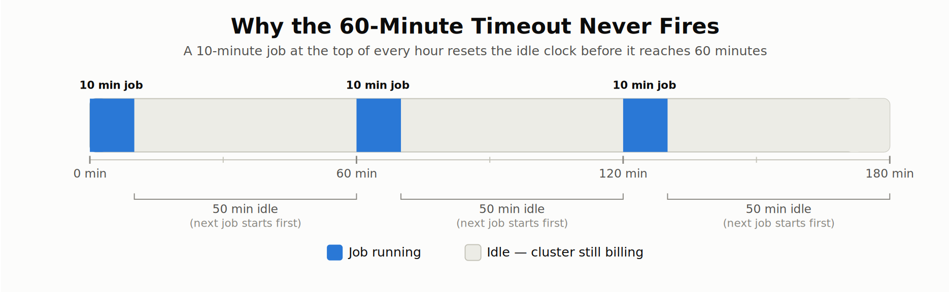
That does not mean shorter inactivity timeouts are always better. If idle gaps are under 10 minutes (the minimum Databricks allows for classic compute auto termination), lowering the timeout will not help much.
Classic clusters also take three to eight minutes to start (this is what we typically observe; it actually varies by cloud, node type, and whether a pool is in play), so even slightly longer gaps may not justify cycling them. For unpredictable workloads, particularly on all-purpose compute and serverless, weigh the cold start and latency costs before tightening the timeout. The goal is not the lowest possible timeout, but the one that minimizes spend (i.e. idle time) without disrupting workloads.
Here is a quick rule of thumb for choosing the right setting:
TABLE: RULE OF THUMB GUIDANCE ON PICKING DATABRICKS AUTO-TERMINATE PERIODS
| Workload shape | What you'd see in the data | Prescription |
|---|---|---|
| Ad-hoc notebook exploration, 1-2 analysts | Gaps of 5-20 min between commands, cluster up all day | 15-20 min. Below 15 mins you pay the 3-8 min restart more often than you save. |
| Shared dev cluster, one time zone | Short gaps 9-6, then dead overnight | 20-30 min + a scheduled terminate at end of day. The timeout handles the daytime tail; only a schedule handles the night. |
| Team split across time zones | Cluster up 18-20 hrs, never idle for 30 min straight | Don't lower the timeout: it will never fire. Split into per-region clusters, or move the workload to a serverless SQL warehouse. |
| Scheduled batch running on all-purpose compute (our 10-min-per-hour example) | Regular short bursts, gaps shorter than the timeout | Wrong lever. Move to job compute, which terminates on completion, so zero idle time. Timeout tuning caps saving at ~50 min/hr; job compute captures the whole thing. |
| Frequent short jobs (every 15-60 min) on job compute | Paying 3-8 min startup on every run | Instance pool, idle-instance auto-termination set just above the gap (Databricks' own example: 20 min for hourly jobs), Min Idle = 0. |
| BI dashboards on a serverless SQL warehouse | Queries clustered in business hours | Auto Stop 10 min (the default). Serverless restarts in seconds, so there's no reason to run higher. UI floor is 5 min; the API goes to 1 min. This is a good approach for a warehouse serving a single scheduled refresh. |
| BI on a pro/classic SQL warehouse | Same pattern, 3-8 min cold start | Default is 45 min. Cut to 20-30. If you're tempted to go lower, that's the signal to move to serverless, not to keep tightening. |
| Structured Streaming using DStreams | Continuous | Set to 0 (no auto-termination). Databricks doesn't report DStream activity, so an auto-terminating cluster can be killed mid-run. |
| Long single-command ML training | One 4-hour cell, no other activity | 10-15 min is safe. The clock measures time since the last command ran, and a running command counts as activity. |
Measuring Idle Share
Idle share = running minutes with no work / total running minutes.
Plotted across those workload shapes, the percentages spread wider than most teams expect.
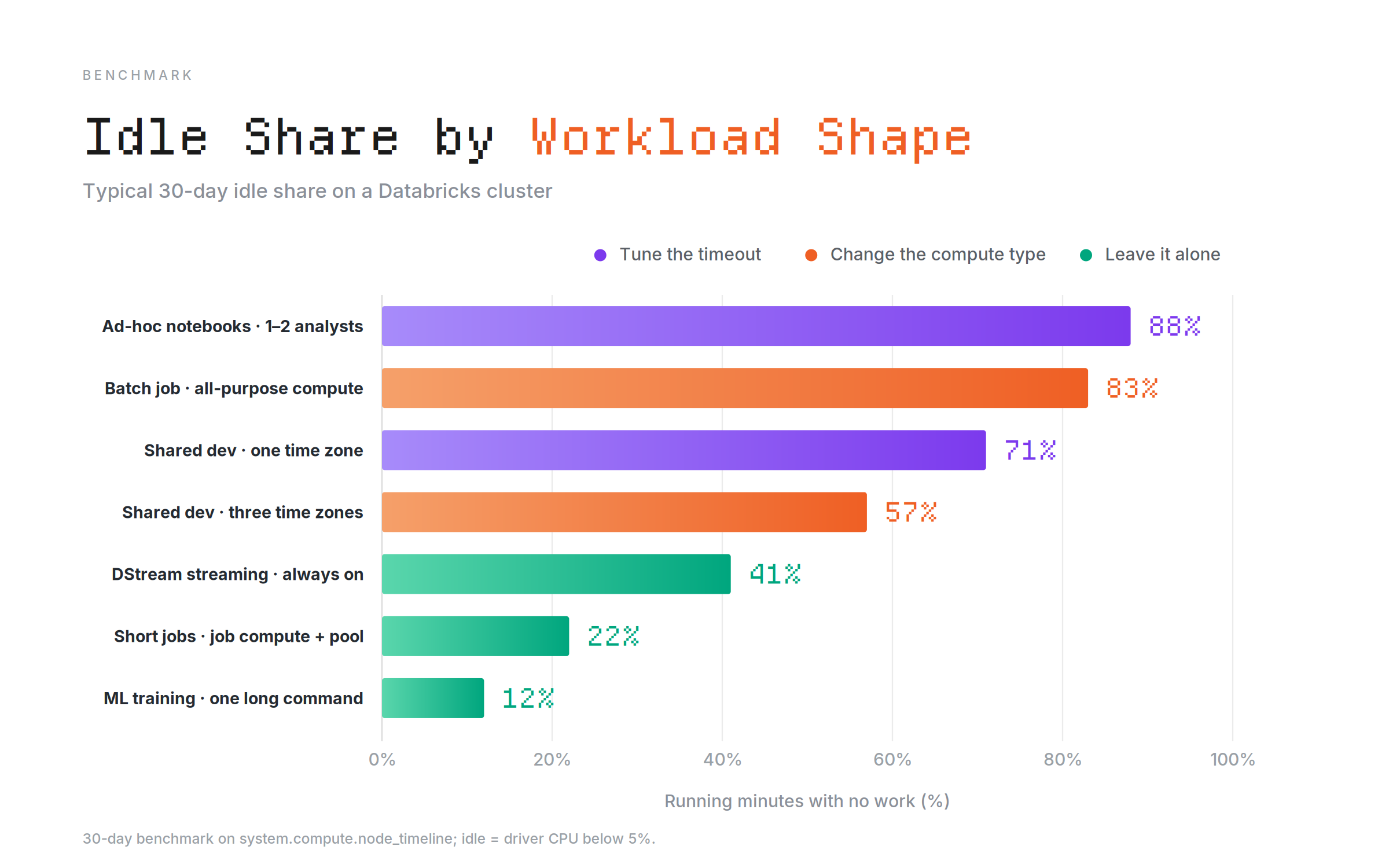
The idle share across the workload shaped in the table above is based on a 30-day benchmark. The percentage alone doesn't tell you the fix: the top two bars waste a similar share of their running time, but one is a timeout problem and the other is a wrong-compute-type problem. SQL warehouses don't appear because of the system.compute.* doesn't cover them.
Streaming shows 41% idle even though the job is live the whole time, because the gaps between micro-batches look like idle minutes to a CPU-based measure. And the query below filters on the driver node, so a cluster with a thin driver and busy executors will report a higher idle share than it deserves. Always check the shape of the workload before you act on the number.
To measure it yourself, over 30 days, per cluster:
SELECT c.cluster_name,
       COUNT(*) AS running_minutes,
       ROUND(100 * SUM(CASE WHEN t.cpu_user_percent + t.cpu_system_percent < 5
                            THEN 1 ELSE 0 END) / COUNT(*), 1) AS pct_idle
FROM system.compute.node_timeline t
JOIN (SELECT DISTINCT cluster_id, cluster_name FROM system.compute.clusters) c
  USING (cluster_id)
WHERE t.start_time >= current_date() - INTERVAL 30 DAYS
  AND t.driver
GROUP BY 1
ORDER BY running_minutes DESC;
Note: system.compute.* excludes SQL warehouses and serverless. Those go through query history and billing tables instead.
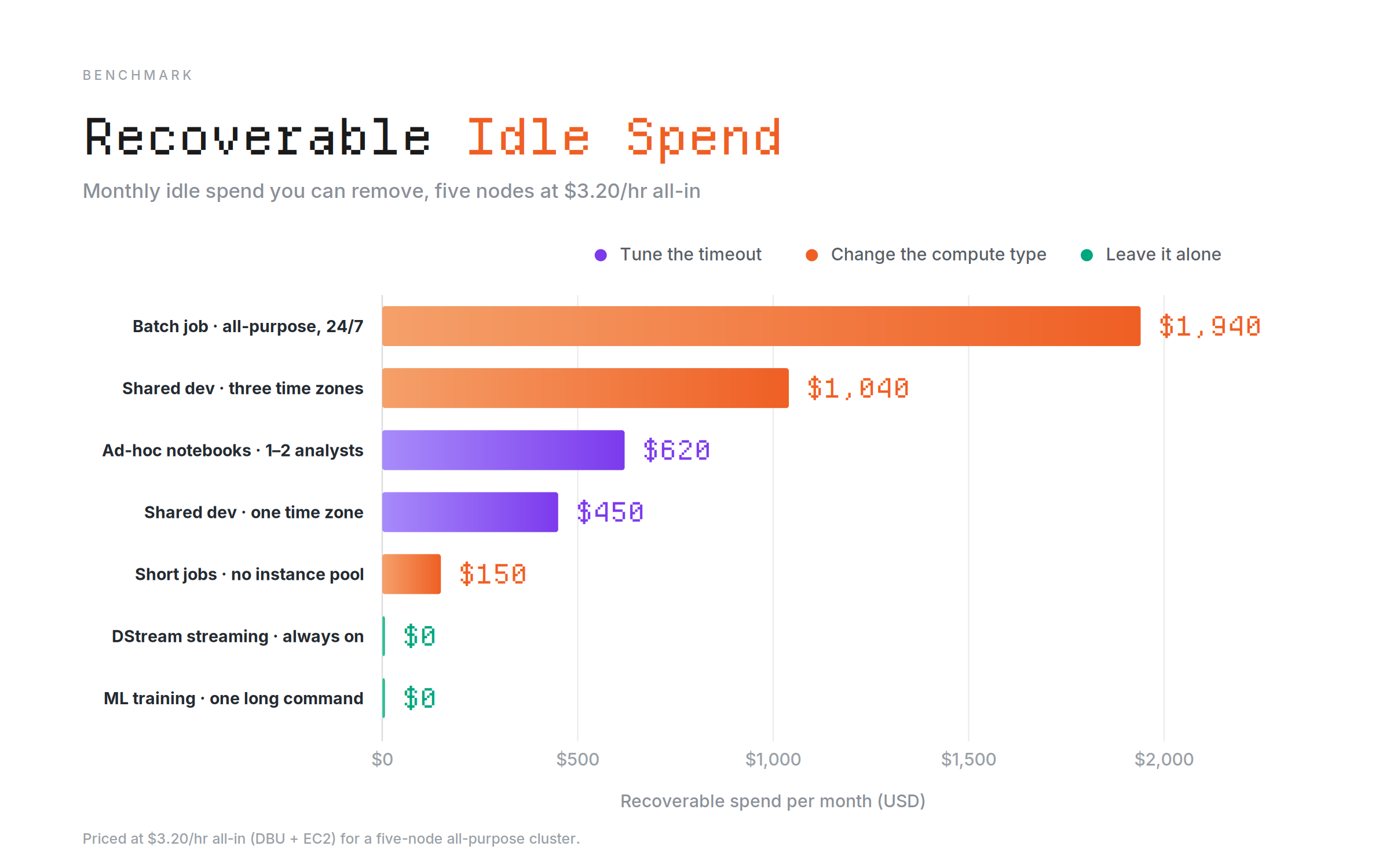
Recoverable idle spend, observed from the same benchmark, is priced at $3.20/hr all-in (DBU + EC2) for a five-node all-purpose cluster. Ad-hoc notebooks have the highest idle share but only the third-largest bill, because a cluster that is up ten hours a day can only waste ten hours a day. Streaming and long training show $0; their idle minutes are real, but there is nothing to reclaim.
This is why idle percentage is a triage signal rather than a priority list. Sort your own query output by running_minutes * pct_idle instead of by pct_idle, and the clusters that are worth fixing first will move to the top of the list.
Finally, constrain autotermination_minutes in a compute policy (range with a max, or fixed + hidden). And audit for the value 0, which means "never terminate".
Cost Lever #4: Size the Driver Independently of the Workers
Sizing the driver is different from tuning the autoscaling range for your worker pool. This lever is about the driver specifically and one that almost nobody touches because Databricks sets the driver node type to match the worker node type by default: "The default value of the driver node type is the same as the worker node type" (Databricks compute configuration docs).
But that default can be wrong in both directions:
Databricks recommends a larger driver when you pull large result sets back using
.collect(), or when multiple notebooks share the same cluster.On the other hand, standard ETL jobs that only transform and write data rarely need large drivers. For those jobs, the default setting forces you to pay for an oversized driver that sits mostly idle.
Always size the driver to match what your specific workload requires rather than trusting the default.
Cost Lever #5: Move Scheduled Databricks Workloads Off All-purpose Clusters
Running production schedules on all-purpose clusters often looks like a scheduling or efficiency issue, but the real driver of the high bill is simply the rate difference. Databricks job compute is typically two to three times cheaper than all-purpose compute. That’s a rule-of-thumb: your actual savings will depend on how long the original cluster sat idle and whether DBUs or raw cloud infrastructure made up the bulk of your costs.
Migrating scheduled workloads off all-purpose clusters onto job compute changes how resources behave. An all-purpose cluster stays warm and ready between runs, whereas a job cluster spins up fresh and shuts down every time. For daily batch runs, accepting that brief cold start is well worth the cost savings. For high-frequency jobs running every few minutes, you have to weigh the startup overhead against the lower compute rates.
Why is My Databricks Production Job Still on an All-purpose Cluster?
Development teams often start their work on an all-purpose cluster because development is interactive by nature. They run a cell, look at the output, change something, and run it again.
Nobody decided production should run on an all-purpose cluster. Production just inherited a decision made in development
Once the things get approved and signed off, they get promoted to a schedule. And the pipeline code that lands in the main branch still points at the same cluster ID or policy it was written against, because when promoting the branch, nobody reviewed its compute config. Nobody decided production should run on an all-purpose cluster. Production just inherited a decision made in development, the same way the driver inherited the worker's size in the last lever.
Auto-termination helps here (see lever 3) but doesn't fix it. It cuts the idle-time waste on that cluster. It doesn't move the job to the compute type that's actually cheaper for the work it's now doing on a schedule.
This is hard to catch by scanning dashboards, because a job on the wrong compute type looks completely healthy. Finding it manually means joining system.billing.usage against system.lakeflow.job_task_run_timeline and asking which production jobs still show up against an all-purpose SKU.
The attribution won't be possible accurately: Databricks says precise cost accounting for jobs sharing all-purpose compute isn't possible with full accuracy, since several workloads draw on the same cluster at once, which is itself an argument for moving the job rather than pricing it after the fact.
Cost Lever #6: Use Spot or Reserved Instances
Spot instances can significantly cut Databricks compute costs, but the cloud provider can reclaim them, so use them for worker nodes, not the driver. If a Spot worker is reclaimed, Spark can retry its tasks elsewhere; if the driver is reclaimed, the entire job fails because the driver coordinates the cluster.
Keep one rule: use spot instances only for worker nodes, and keep your driver node on standard on-demand compute.
On AWS, use fleet instance types so Databricks can choose from multiple instance types based on availability and price, rather than relying on a single type that may not be available when you need it.
For predictable workloads, Reserved Instances (RIs) have huge CUDs (Committed Use Discounts) and can provide significant savings without Spot's interruption risk. Use Spot when your workload can tolerate worker replacement; use RIs when you need consistent capacity and predictable savings.
Both Spot and RIs reduce the cloud VM cost, not DBUs. This makes them more impactful for job compute, where infrastructure is a larger share of the bill, than for all-purpose compute, where DBUs typically are a larger share of the total bill. Know which area of the bill you're attacking before you decide to go for spot instances or RIs.
When Databricks Spot Compute is the wrong call,
Spot is good where interruption is tolerable: retry-friendly batch ETL, checkpointed pipelines, and fault-tolerant model training. Conversely, a low-latency dashboard query or an SLA-bound job is the wrong place to try your first spot rollout.
Databricks Auto Tune: Put Optimization on Autopilot
Now that we have seen all these 6 levers, it comes down to executing and running a cost reduction sprint within the team and getting those levers set to their optimum position. However, getting them right once doesn’t guarantee value over time; these levers need to be adjusted every now and then, as the demands and requirements change. Constantly keeping them in check requires time and effort
The Altimate Platform provides precisely such a feature called Auto Tune, which automatically sets all six levers we discussed (with safe configuration backoff), going well beyond Databrick’s Predictive Optimization.
How Altimate Auto Tune Automatically Pulls Levers
Auto Tune analyzes how each SQL warehouse, cluster job, and other workloads are actually used. Including CPU, memory, and worker utilization across recent runs, and then right-sizing things such as
Worker instance type: moving workers to a cheaper, better-fitting family if the current one is over-provisioned.
Driver instance type: right-sized as per need from historic data, since drivers are frequently much larger than the workload requires.
Worker count / autoscaling bounds: tightens a fixed count or the min-max range so the cluster never runs more workers than the job needs.
It only changes the configuration; the code, schedule, tasks, libraries, and tags are never touched. The diagram below gives you a quick overview of how Auto Tune works:

For more information on how you can save more with the Altimate Platform, see Databricks Cost Optimization.
Below are some of the use cases and screenshots of the levers we discussed being used in action and actually providing real cost savings. In the Auto Tune settings page, you can see how it proposes the correct family and instance type by observing the workload and requirements, giving you cost-saving options if you choose to go with that setting.
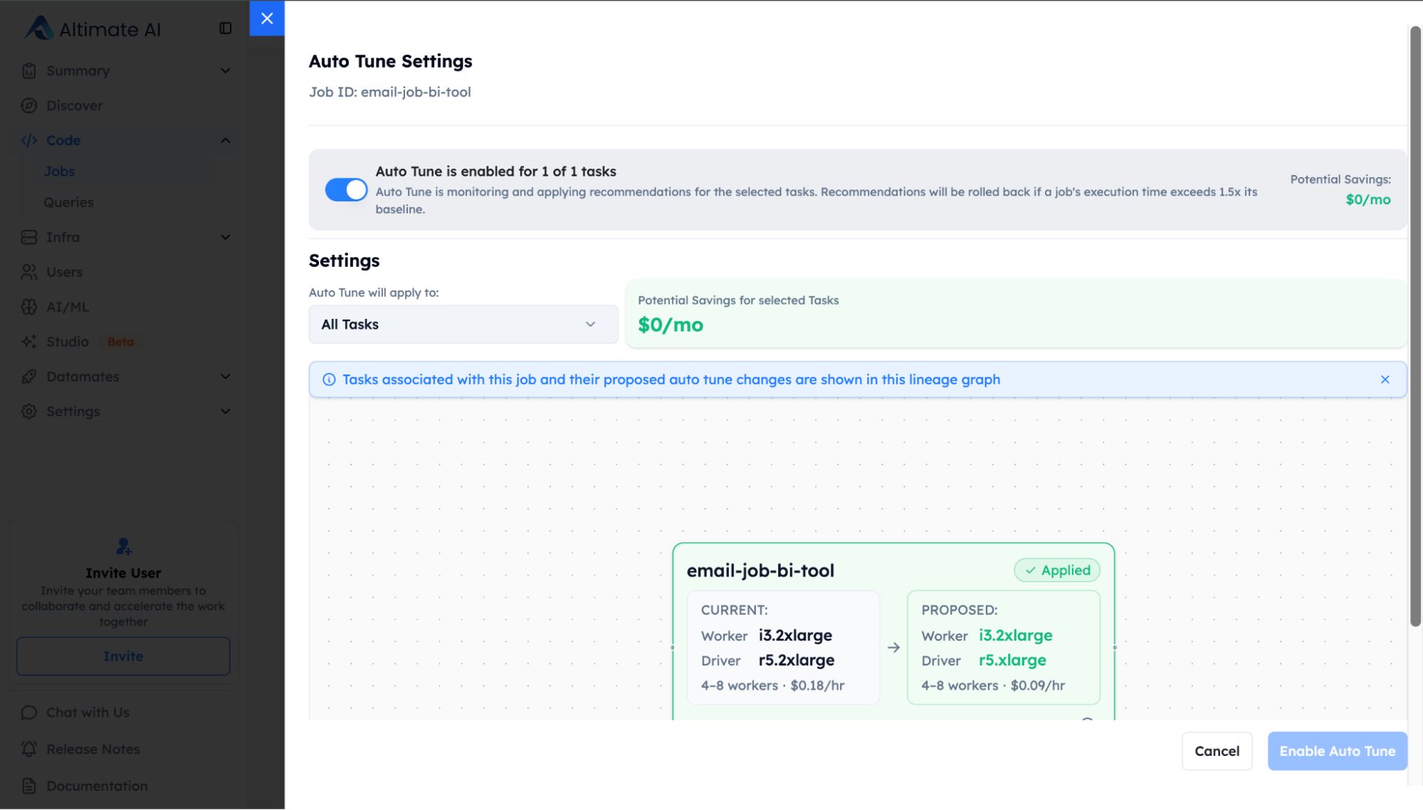
A screenshot of the Altimate UI, a platform that provides cost intelligence and governance for modern data teams. Altimate analyzes actual workload behavior to detect when a job is running on the suboptimal compute family. It provides you with visibility into where the mismatch exists, so you can trust the system's recommendations and decisions.
We previously discussed how Databricks production jobs sometimes keep on running on an all-purpose cluster, and we often miss them because they work just fine; they just cost way more than they should.
This issue becomes immediately visible with Altimate’s “discover” tab:
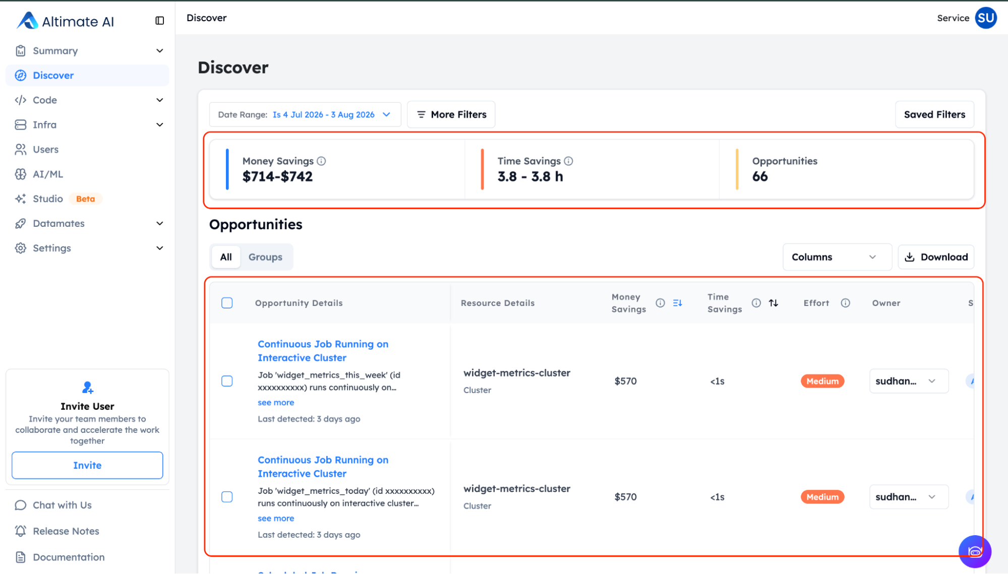
The Discover page in the Altimate.ai enterprise platform runs a version of that system.billing.usage against system.lakeflow.job_task_run_timeline join continuously and surfaces exactly this pattern: a job still running on an interactive cluster long after the workload stopped being interactive, flagged with the switch to make and the same accuracy limit attached.
Further information on the Altimate Platform can be found in Databricks Cost Optimization, or if you use Snowflake, read Adaptive Compute vs. Altimate AI Auto Tune Optimization
If you want to explore Altimate, you can book some time with the team here.
Conclusion
Hopefully, this blog post leaves you with a direct answer as to what actually reduces Databricks compute costs. We’ve highlighted six levers that can make the biggest difference and should be your first focus. There are certainly other levers you can pull to bring your Databricks costs down. The key is knowing where to look and which ones are likely to have the biggest impact.
TABLE: Summary of the Main 6 Levers to Cost Optimization on Databricks
The details shared in this table don't show up in a rate calculator because they're behavior and configuration decisions, not billing rates. They decide how much of that calculated hourly number you actually end up paying for.
Note on the savings column below: ranges are directional and apply to the workload not to your whole bill. Treat them the way we treated the auto-terminate example: useful for prioritizing, but not a quote. In our experience, teams that work through all six typically land in the 20-35% range on total Databricks compute spend.
| Lever | Setting to change | What you give up | Which half of the bill is improved (DBU or Infra) | Typical savings (directional, on the affected workload) |
|---|---|---|---|---|
| 1) Match compute type to workload | Serverless or classic, per workload shape | Spot pricing, on anything you move to serverless | DBU | 50-75% of a bursty cluster's cost when utilization was under 25% |
| 2) Turn on Photon where it applies | Photon toggle on the cluster or warehouse | Nothing if it's out of scope, but you pay the higher Photon rate for no speedup | DBU | Turning Photon off where it adds no value -> up to roughly half that job's DBU line on classic compute. |
| 3) Tighten auto-termination | Auto-terminate minutes | Cold-start waits, and the risk people leave clusters up to avoid them | Both | 20-40% of classic compute spend |
| 4) Size the driver for its job | Driver node type, unpinned from the worker type | A bigger driver costs more; too small and .collect() fails the job | Infrastructure, mostly | Single-digit % of that cluster's infra bill |
| 5) Move scheduled work to job compute | Cluster type on the job definition | The warm interactive session the notebook was developed against | DBU | 40-60% off that job's total cost. |
| 6) Spot workers, on-demand driver | Spot for workers, Fleet types on AWS, driver stays on-demand | Interruption tolerance, so not for SLA-bound work | Infrastructure only | 60-90% off the workers' VM price (DBUs unchanged) |
For the two-bill split and the system tables behind all six, see our blog post, Understanding Databricks Compute Costs.